Analyzing a set of observations in a loop#
When a star has multiple observations, it is useful to make a loop over all of the spectra files rather than running each one individually. To obtain LSD profiles and \(B_z\) values, only one cleaned line mask is necessary since all the spectra files are from the same star. With the cleaned mask and .s files, you can loop over the run_lsdpy function to calculate outputs for each input spectrum file.
In the below tutorial, we will walk through how to calculate data from multiple spectra files for the same star. It is recommended you first look through the tutorial for analyzing one observation for additional background on individual steps. We have provided three spectra files: hd46328_test_1.s, hd46328_test_2.s, and hd46328_test_3.s for \(\xi^1\) CMa (HD 46328; Erba et al. 2021) and the line list (LongList_T27000G35.dat) from the Vienna Atomic Line Database (VALD; Ryabchikova et al. 2015).
First import specpolFlow and any other packages
1. Normalize the spectra#
Before running LSD, the observed spectra need to be reasonably well normalized. In some cases an automatic pipeline normalization might be sufficient. For a more careful manual normalization, we can use normPlot. When there are multiple observations of the same star made with the same instrument, a good approach can be to carefully normalize one observation, then save the parameters from normPlot and reuse those for the rest of the observations.
That approach is illustrated here, although the example spectra are already relatively well normalized (except around the edges of a few spectral orders).
To normalize the first observation, you can follow the normPlot guide. Don’t forget to click the “save params” button before exiting!
# to run normPlot from within Python
import normPlot
normPlot.normplot('OneObservationFlow_tutorialfiles/hd46328_test_1.s')

# or to run normPlot from the terminal use
# normplot OneObservationFlow_tutorialfiles/hd46328_test_1.s
If you clicked the “save params” button, the parameters from normalizing the first observation will be saved to the files exclude.dat, poly-deg.dat, and params.dat. These can then be applied to all the other observations. Here we run normPlot in a loop, and use batchMode=True to skip the graphical interface.
obsfile_list = ['OneObservationFlow_tutorialfiles/hd46328_test_1.s',
                'OneObservationFlow_tutorialfiles/hd46328_test_2.s',
                'OneObservationFlow_tutorialfiles/hd46328_test_3.s']
for file in obsfile_list:
    normPlot.normplot(file, excludeRegionName='exclude.dat',
                      polynomialsName='poly-deg.dat',
                      paramsName='params.dat', batchMode=True)
This generates a set of files (OneObservationFlow_tutorialfiles/hd46328_test_1.s.norm, OneObservationFlow_tutorialfiles/hd46328_test_2.s.norm, OneObservationFlow_tutorialfiles/hd46328_test_3.s.norm). These should have a consistent normalization, and can be used for the rest of the tutorial. However, to keep this step optional, and since the initial files were adequately normalized, we use the originals to calculate LSD profiles below.
2. Create & clean the LSD line mask#
Since all our observations are of the same star, we can create one mask that can be used for all the observations of the star. We specify the name of the VALD line list and the name and location of our created mask. Next, we remove regions within 300 km s\(^{-1}\) (specific to this example) of the Balmer series and Balmer jump.
# making the mask file from the VALD line list
lineList_filename = 'OneObservationFlow_tutorialfiles/LongList_T27000G35.dat'
full_mask_filename = 'OneObservationFlow_tutorialfiles/test_output/T27000G35_depth0.02.mask'
mask = pol.make_mask(lineList_filename, outMaskName=full_mask_filename, depthCutoff = 0.02, atomsOnly = True)

# using default regions for cleaning
velrange = 300.0
ExcludeRegions = pol.get_Balmer_regions_default(velrange) + pol.get_telluric_regions_default()

# cleaning and saving the mask
clean_mask_filename = 'OneObservationFlow_tutorialfiles/test_output/hd46328_test_depth0.02_clean.mask'
mask.clean(ExcludeRegions).save(clean_mask_filename)

# optionally, you can interactively clean lines from the line mask with
# pol.cleanMaskUI(full_mask_filename, observation_filename, clean_mask_filename)
missing Lande factors for 160 lines (skipped) from:
['He 2', 'O 2']
skipped all lines for species:
['H 1']
To fine-tune the mask, it can be helpful to use the interactive mask cleaning tool. See the full tutorial for more information.
3. Create LSD profile#
We then create the LSD profiles for all three observed spectra files, by looping over the file names of the observations and running LSDpy.
obsfile_list = ['OneObservationFlow_tutorialfiles/hd46328_test_1.s',
                'OneObservationFlow_tutorialfiles/hd46328_test_2.s',
                'OneObservationFlow_tutorialfiles/hd46328_test_3.s']

for obsfile in obsfile_list:
    # Generate a name for the LSD profile, in a different folder.
    # This could also just be pulled from a list of output file names.
    lsdfile = obsfile.replace('tutorialfiles/','tutorialfiles/test_output/').replace('.s', '.lsd')
    lsd, mod = pol.run_lsdpy(obs = obsfile,
            mask = clean_mask_filename, outLSDName = lsdfile,
            velStart = - 100.0, velEnd = 100.0, velPixel = 2.6,
            normDepth = 0.2, normLande = 1.2, normWave = 500.0,
            plotLSD=False)
Modified line mask, removed 75 too closely spaced lines
Average observed spec velocity spacing: 1.810029 km/s
using a 78 point profile with 2.600000 km/s pixels
mean mask depth 0.102471 wl 494.041 Lande 1.180924 (from 1028 lines)
mean mask norm weightI 0.512354 weightV 0.485692
saving model spectrum to  ...
I reduced chi2 263.1932 (chi2 20377468.87 constraints 77502 dof 78)
 Rescaling error bars by: 16.223230
V reduced chi2 1.1246 (chi2 87074.15 constraints 77502 dof 78)
 Rescaling error bars by: 1.060491
 removing profile continuum pol: -8.3777e-06 +/- 8.4331e-09 (avg err 9.1553e-05)
N1 reduced chi2 1.1030 (chi2 85396.51 constraints 77502 dof 78)
 Rescaling error bars by: 1.050225
 removing profile continuum pol: -9.2523e-07 +/- 8.2706e-09 (avg err 9.0667e-05)
(possible Stokes I uncertainty underestimate 1.9564e-03 vs 1.4637e-03)
line range estimate -14.200000000000188 42.99999999999969 km/s
V in line reduced chi^2 92.046659 (chi2 2025.026499)
 detect prob 1.000000 (fap 0.000000e+00)
 Detection! V (fap 0.000000e+00)
 V outside line reduced chi^2 1.635616 (chi2  81.780822)
 detect prob 0.996959 (fap 3.041463e-03)
N1 in line reduced chi^2 1.028558 (chi2  22.628284)
 detect prob 0.577033 (fap 4.229666e-01)
 Non-detection N1 (fap 4.229666e-01)
 N1 outside line reduced chi^2 0.967249 (chi2  48.362446)
 detect prob 0.460702 (fap 5.392980e-01)
Modified line mask, removed 75 too closely spaced lines
Average observed spec velocity spacing: 1.810124 km/s
using a 78 point profile with 2.600000 km/s pixels
mean mask depth 0.102471 wl 494.041 Lande 1.180924 (from 1028 lines)
mean mask norm weightI 0.512354 weightV 0.485692
saving model spectrum to  ...
I reduced chi2 234.5534 (chi2 18161704.65 constraints 77509 dof 78)
 Rescaling error bars by: 15.315136
V reduced chi2 1.1182 (chi2 86581.50 constraints 77509 dof 78)
 Rescaling error bars by: 1.057439
 removing profile continuum pol: -1.6806e-05 +/- 8.3843e-09 (avg err 9.1340e-05)
N1 reduced chi2 1.1060 (chi2 85641.85 constraints 77509 dof 78)
 Rescaling error bars by: 1.051685
 removing profile continuum pol: -1.2960e-05 +/- 8.2933e-09 (avg err 9.0843e-05)
(possible Stokes I uncertainty underestimate 2.3769e-02 vs 1.3604e-03)
line range estimate 37.7999999999997 45.59999999999968 km/s
V in line reduced chi^2 17.855157 (chi2  53.565470)
 detect prob 1.000000 (fap 1.388933e-11)
 Detection! V (fap 1.388933e-11)
 V outside line reduced chi^2 47.448111 (chi2 3273.919664)
 detect prob 1.000000 (fap 0.000000e+00)
N1 in line reduced chi^2 0.897654 (chi2   2.692961)
 detect prob 0.558575 (fap 4.414248e-01)
 Non-detection N1 (fap 4.414248e-01)
 N1 outside line reduced chi^2 1.115116 (chi2  76.943019)
 detect prob 0.760555 (fap 2.394452e-01)
Modified line mask, removed 75 too closely spaced lines
Average observed spec velocity spacing: 1.810284 km/s
using a 78 point profile with 2.600000 km/s pixels
mean mask depth 0.102471 wl 494.041 Lande 1.180924 (from 1028 lines)
mean mask norm weightI 0.512354 weightV 0.485692
saving model spectrum to  ...
I reduced chi2 260.5906 (chi2 20176227.04 constraints 77503 dof 78)
 Rescaling error bars by: 16.142819
V reduced chi2 1.1432 (chi2 88515.87 constraints 77503 dof 78)
 Rescaling error bars by: 1.069227
 removing profile continuum pol: -4.1582e-06 +/- 8.9941e-09 (avg err 9.4554e-05)
N1 reduced chi2 1.1114 (chi2 86046.37 constraints 77503 dof 78)
 Rescaling error bars by: 1.054206
 removing profile continuum pol: -7.9709e-06 +/- 8.7431e-09 (avg err 9.3226e-05)
(possible Stokes I uncertainty underestimate 2.6324e-03 vs 1.4916e-03)
line range estimate -6.400000000000205 42.99999999999969 km/s
V in line reduced chi^2 105.945743 (chi2 2012.969113)
 detect prob 1.000000 (fap 0.000000e+00)
 Detection! V (fap 0.000000e+00)
 V outside line reduced chi^2 2.022796 (chi2 107.208182)
 detect prob 0.999985 (fap 1.536931e-05)
N1 in line reduced chi^2 1.127698 (chi2  21.426269)
 detect prob 0.686268 (fap 3.137322e-01)
 Non-detection N1 (fap 3.137322e-01)
 N1 outside line reduced chi^2 1.244780 (chi2  65.973366)
 detect prob 0.891292 (fap 1.087085e-01)
We can also generate all the file names inside a loop using a template string:
# create a template for the filenames
obsfile = 'OneObservationFlow_tutorialfiles/hd46328_test_{}.s'
lsdfile = 'OneObservationFlow_tutorialfiles/test_output/hd46328_test_{}.lsd'

for i in range(3):
    # here we generate file names from a template
    lsd, mod = pol.run_lsdpy(obs = obsfile.format(i+1),
            mask = clean_mask_filename, outLSDName = lsdfile.format(i+1),
            velStart = - 100.0, velEnd = 100.0, velPixel = 2.6,
            normDepth = 0.2, normLande = 1.2, normWave = 500.0,
            plotLSD=False)
Modified line mask, removed 75 too closely spaced lines
Average observed spec velocity spacing: 1.810029 km/s
using a 78 point profile with 2.600000 km/s pixels
mean mask depth 0.102471 wl 494.041 Lande 1.180924 (from 1028 lines)
mean mask norm weightI 0.512354 weightV 0.485692
saving model spectrum to  ...
I reduced chi2 263.1932 (chi2 20377468.87 constraints 77502 dof 78)
 Rescaling error bars by: 16.223230
V reduced chi2 1.1246 (chi2 87074.15 constraints 77502 dof 78)
 Rescaling error bars by: 1.060491
 removing profile continuum pol: -8.3777e-06 +/- 8.4331e-09 (avg err 9.1553e-05)
N1 reduced chi2 1.1030 (chi2 85396.51 constraints 77502 dof 78)
 Rescaling error bars by: 1.050225
 removing profile continuum pol: -9.2523e-07 +/- 8.2706e-09 (avg err 9.0667e-05)
(possible Stokes I uncertainty underestimate 1.9564e-03 vs 1.4637e-03)
line range estimate -14.200000000000188 42.99999999999969 km/s
V in line reduced chi^2 92.046659 (chi2 2025.026499)
 detect prob 1.000000 (fap 0.000000e+00)
 Detection! V (fap 0.000000e+00)
 V outside line reduced chi^2 1.635616 (chi2  81.780822)
 detect prob 0.996959 (fap 3.041463e-03)
N1 in line reduced chi^2 1.028558 (chi2  22.628284)
 detect prob 0.577033 (fap 4.229666e-01)
 Non-detection N1 (fap 4.229666e-01)
 N1 outside line reduced chi^2 0.967249 (chi2  48.362446)
 detect prob 0.460702 (fap 5.392980e-01)
Modified line mask, removed 75 too closely spaced lines
Average observed spec velocity spacing: 1.810124 km/s
using a 78 point profile with 2.600000 km/s pixels
mean mask depth 0.102471 wl 494.041 Lande 1.180924 (from 1028 lines)
mean mask norm weightI 0.512354 weightV 0.485692
saving model spectrum to  ...
I reduced chi2 234.5534 (chi2 18161704.65 constraints 77509 dof 78)
 Rescaling error bars by: 15.315136
V reduced chi2 1.1182 (chi2 86581.50 constraints 77509 dof 78)
 Rescaling error bars by: 1.057439
 removing profile continuum pol: -1.6806e-05 +/- 8.3843e-09 (avg err 9.1340e-05)
N1 reduced chi2 1.1060 (chi2 85641.85 constraints 77509 dof 78)
 Rescaling error bars by: 1.051685
 removing profile continuum pol: -1.2960e-05 +/- 8.2933e-09 (avg err 9.0843e-05)
(possible Stokes I uncertainty underestimate 2.3769e-02 vs 1.3604e-03)
line range estimate 37.7999999999997 45.59999999999968 km/s
V in line reduced chi^2 17.855157 (chi2  53.565470)
 detect prob 1.000000 (fap 1.388933e-11)
 Detection! V (fap 1.388933e-11)
 V outside line reduced chi^2 47.448111 (chi2 3273.919664)
 detect prob 1.000000 (fap 0.000000e+00)
N1 in line reduced chi^2 0.897654 (chi2   2.692961)
 detect prob 0.558575 (fap 4.414248e-01)
 Non-detection N1 (fap 4.414248e-01)
 N1 outside line reduced chi^2 1.115116 (chi2  76.943019)
 detect prob 0.760555 (fap 2.394452e-01)
Modified line mask, removed 75 too closely spaced lines
Average observed spec velocity spacing: 1.810284 km/s
using a 78 point profile with 2.600000 km/s pixels
mean mask depth 0.102471 wl 494.041 Lande 1.180924 (from 1028 lines)
mean mask norm weightI 0.512354 weightV 0.485692
saving model spectrum to  ...
I reduced chi2 260.5906 (chi2 20176227.04 constraints 77503 dof 78)
 Rescaling error bars by: 16.142819
V reduced chi2 1.1432 (chi2 88515.87 constraints 77503 dof 78)
 Rescaling error bars by: 1.069227
 removing profile continuum pol: -4.1582e-06 +/- 8.9941e-09 (avg err 9.4554e-05)
N1 reduced chi2 1.1114 (chi2 86046.37 constraints 77503 dof 78)
 Rescaling error bars by: 1.054206
 removing profile continuum pol: -7.9709e-06 +/- 8.7431e-09 (avg err 9.3226e-05)
(possible Stokes I uncertainty underestimate 2.6324e-03 vs 1.4916e-03)
line range estimate -6.400000000000205 42.99999999999969 km/s
V in line reduced chi^2 105.945743 (chi2 2012.969113)
 detect prob 1.000000 (fap 0.000000e+00)
 Detection! V (fap 0.000000e+00)
 V outside line reduced chi^2 2.022796 (chi2 107.208182)
 detect prob 0.999985 (fap 1.536931e-05)
N1 in line reduced chi^2 1.127698 (chi2  21.426269)
 detect prob 0.686268 (fap 3.137322e-01)
 Non-detection N1 (fap 3.137322e-01)
 N1 outside line reduced chi^2 1.244780 (chi2  65.973366)
 detect prob 0.891292 (fap 1.087085e-01)
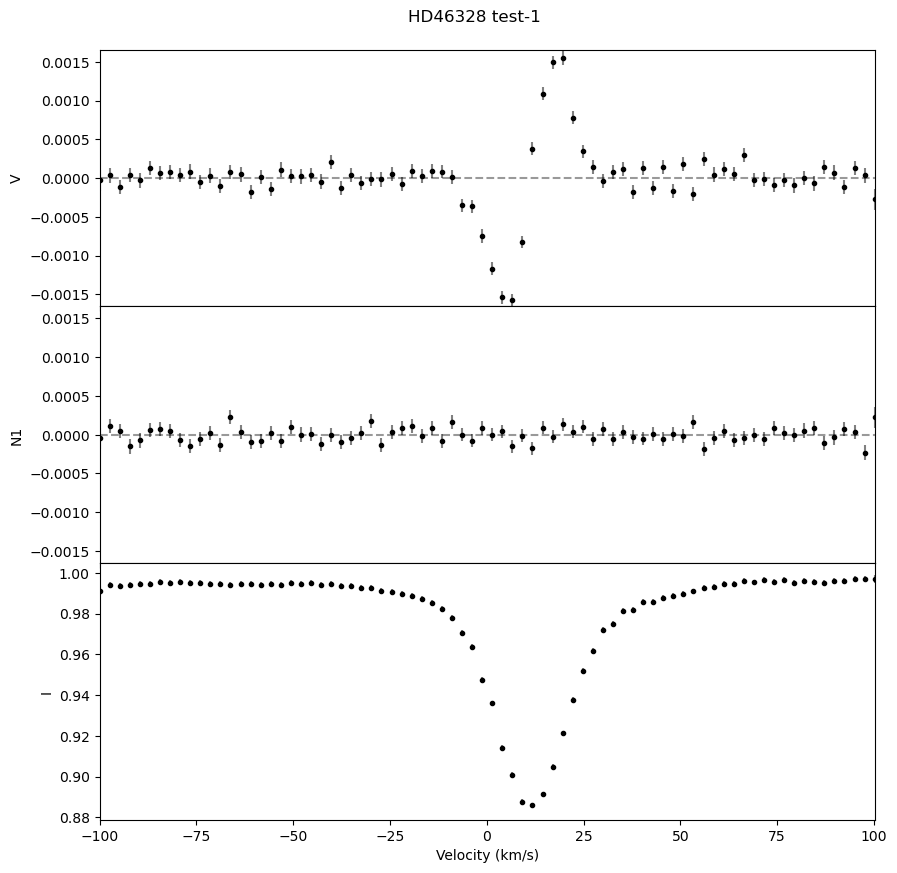
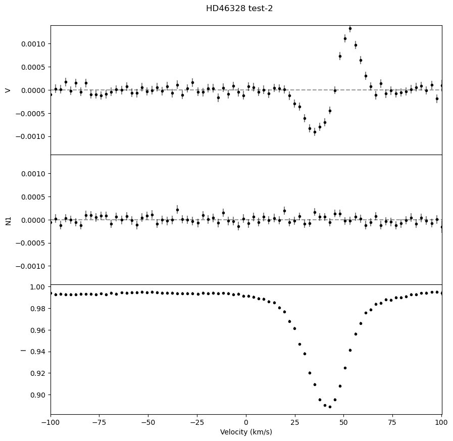
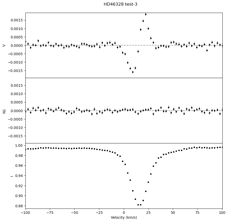
We can also output a .pdf with plots of the LSD profiles for each observation, which is useful for ensuring that the LSD profiles look as expected.
# open an output .pdf file
with PdfPages('OneObservationFlow_tutorialfiles/test_output/hd46328_test.pdf') as pdf:
    lsdfile = 'OneObservationFlow_tutorialfiles/test_output/hd46328_test_{}.lsd'
    # loop over the LSD profiles, reading them in and plotting them
    for i in range(3):
        lsd = pol.read_lsd(lsdfile.format(i+1))
        fig, ax = lsd.plot()

        fig.suptitle('HD46328 test' + '-'+ str(i+1), y = 0.92)
        pdf.savefig(fig)
4. Bz calculation#
We can then loop over the LSD profiles to calculate Bz for each of them. In this example, each observation has a different radial velocity. This means the integration range used in the Bz calculation needs to be different for each observation. (For a normal sincle star this is not necessary). One method to resolve this is to make a list of vrad values, and use those inside the loop.
# create a template for the LSD profile filenames
lsdpath = 'OneObservationFlow_tutorialfiles/test_output/hd46328_test_{}.lsd'

# set the radial velocity for each observation
vrad = [12.0, 42.0, 16.0]

# save the results into a list, appending to the list
Bz_list = []
for i in range(3):
    velrange = [vrad[i] - 30.0, vrad[i] + 30.0]

    # read the LSD profile
    lsd = pol.read_lsd(lsdpath.format(i+1))

    # calculate Bz, using the velocity range set for this observation
    Bz = lsd.calc_bz(cog = 'I', velrange = velrange, bzwidth = 20.0, plot = False)
    Bz_list.append(Bz)

# print some results
for Bz in Bz_list:
    print('V bz (G)', Bz['V bz (G)'], ' V bz sig (G)', Bz['V bz sig (G)'], ' V FAP', Bz['V FAP'])
using AUTO method for the normalization
  using the median of the continuum outside of the line
using AUTO method for the normalization
  using the median of the continuum outside of the line
using AUTO method for the normalization
  using the median of the continuum outside of the line
V bz (G) -113.65424816561506  V bz sig (G) 4.148373089850504  V FAP 0.0
V bz (G) -112.49569214929704  V bz sig (G) 4.409081202807453  V FAP 0.0
V bz (G) -104.44383156707192  V bz sig (G) 4.2734725037558965  V FAP 0.0
Often, we want to output a single table with the Bz results for all observations. This can be done conveniently with pandas. A reasonably efficient approach is to collect the results for each observation into a list, then make a dataframe from that list. Alternatively, one could incrementally add to a dataframe on each iteration of the loop (e.g. table = pd.concat(table, newline)), although this generates new dataframes on each iteration, which is inefficent for large datasets.
Bz_table = pd.DataFrame(Bz_list)

star = ['hd46328_1', 'hd46328_2', 'hd46328_3']
Bz_table.insert(0, "Star", star)

Bz_table
| Star | V bz (G) | V bz sig (G) | V FAP | N1 bz (G) | N1 bz sig (G) | N1 FAP | N2 bz (G) | N2 bz sig (G) | N2 FAP | norm_method | norm | cog_method | cog | int. range start | int. range end | |
|---|---|---|---|---|---|---|---|---|---|---|---|---|---|---|---|---|
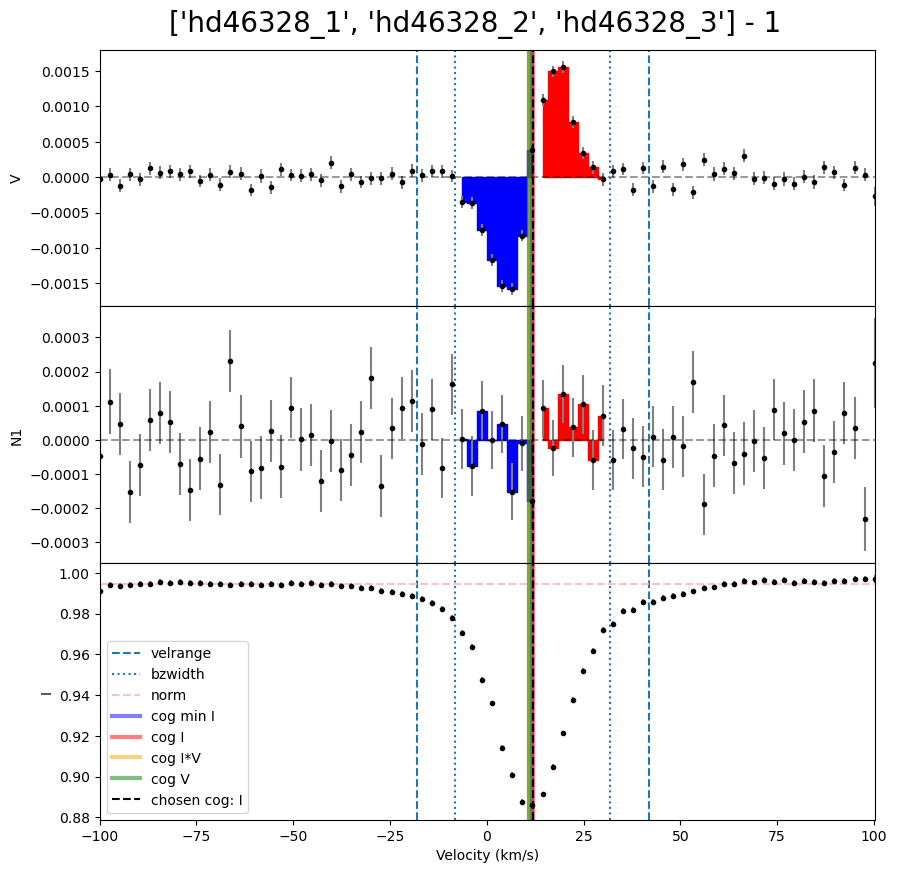
| 0 | hd46328_1 | -113.654248 | 4.148373 | 0.0 | -3.967533 | 4.065204 | 0.281862 | 0.0 | 0.0 | 0.0 | auto | 0.994433 | I | 11.836342 | -8.163658 | 31.836342 |
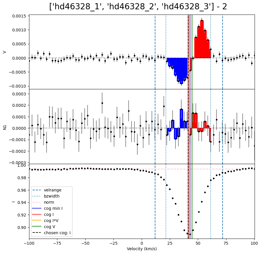
| 1 | hd46328_2 | -112.495692 | 4.409081 | 0.0 | -1.465655 | 4.350233 | 0.411965 | 0.0 | 0.0 | 0.0 | auto | 0.993514 | I | 41.379051 | 21.379051 | 61.379051 |
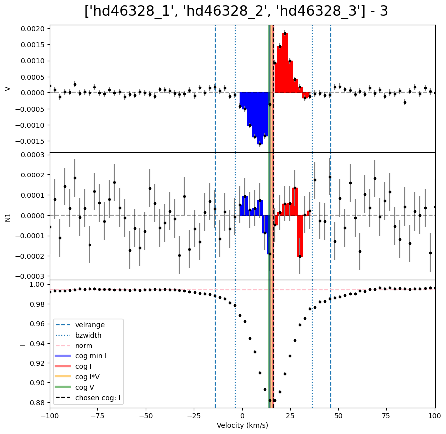
| 2 | hd46328_3 | -104.443832 | 4.273473 | 0.0 | 3.006969 | 4.177154 | 0.249865 | 0.0 | 0.0 | 0.0 | auto | 0.994229 | I | 16.425263 | -3.574737 | 36.425263 |
As before, we can also make a .pdf for all the Bz plots. Here we repeat the previous steps and generate a ‘.pdf’ with the Bz plots.
lsdpath = 'OneObservationFlow_tutorialfiles/test_output/hd46328_test_{}.lsd'
vrad = [12.0, 42.0, 16.0]
star = ['hd46328_1', 'hd46328_2', 'hd46328_3']

with PdfPages('OneObservationFlow_tutorialfiles/test_output/hd46328_test_Bz.pdf') as pdf:

    Bz_list = []
    for i in range(3):
        lsd = pol.read_lsd(lsdpath.format(i+1))

        velrange = [vrad[i] - 30.0, vrad[i] + 30.0]
        Bz, fig = lsd.calc_bz(cog = 'I', velrange = velrange, bzwidth = 20.0, plot = True)
        Bz_list.append(Bz)

        fig.suptitle('{} - {}'.format(star,i+1), fontsize = 20, y = 0.92)
        pdf.savefig(fig)

Bz_table = pd.DataFrame(Bz_list)
Bz_table.insert(0, "Star", star)
Bz_table