How to compute LSD profiles

How to compute LSD profiles#

In this tutorial, we demonstrate the calculation of LSD profiles using the run_lsdpy function, which is a wrapper around the main function of the LSDpy Package.

The advantage of the run_lsdpy function is that it has been designed with default options that make it easy to use in interactive shells and within python scripts.

Warning

You can of course use the LSDpy.lsd() function directly – however it has different input requirements. It requires all parameters to be passed explicitly or it will default to reading missing parameters from an input file inlsd.dat. This is better suited for a command-line workflow, see Using the command line for details.

To begin, we need to import specpolFlow.

In this tutorial, we assume that you already have a normalized spectrum in a .s format and a mask file that has been suitably cleaned for your needs.

We will use these two files hd46328_test_1.s.norm and hd46328_test_depth0.02_clean.mask

No normalized .s file?

See the following tutorials

No mask file?

See the walkthrough in From normalized spectrum to Bz measurement, and also the following tutorials

In the cell below, we set some variables with the path/name of the observation file and the mask file.

mask_file = 'HowToLSD_tutorialfiles/hd46328_test_depth0.02_clean.mask'
obs_file  = 'HowToLSD_tutorialfiles/hd46328_test_1.s.norm'

1. Calculating an LSD profile “on-the-fly”#

The following section demonstrates a very simple application of the run_lsdpy function.

Note

The run_lsdpy function returns 2 Python objects:

An LSD with the computed LSD profile
A Spectrum object with the LSD model spectrum (more on this later)

In the example below, we have unpacked the returned tuple into two separate variables.

lsd, mod = pol.run_lsdpy(obs=obs_file, mask=mask_file)

Modified line mask, removed 64 too closely spaced lines
Average observed spec velocity spacing: 1.810029 km/s
using a 222 point profile with 1.810000 km/s pixels
mean mask depth 0.101386 wl 494.081 Lande 1.179956 (from 1039 lines)
mean mask norm weightI 0.506930 weightV 0.480710
saving model spectrum to  ...
I reduced chi2 193.8252 (chi2 19858356.38 constraints 102677 dof 222)
 Rescaling error bars by: 13.922110
V reduced chi2 1.1163 (chi2 114372.85 constraints 102677 dof 222)
 Rescaling error bars by: 1.056562
 removing profile continuum pol: -5.3633e-06 +/- 1.2232e-08 (avg err 1.1045e-04)
N1 reduced chi2 1.1078 (chi2 113495.43 constraints 102677 dof 222)
 Rescaling error bars by: 1.052501
 removing profile continuum pol: -6.5530e-06 +/- 1.2138e-08 (avg err 1.1003e-04)
line range estimate -20.809999999999775 49.780000000000314 km/s
V in line reduced chi^2 51.897682 (chi2 2024.009582) 
 detect prob 1.000000 (fap 0.000000e+00)
 Detection! V (fap 0.000000e+00)
 V outside line reduced chi^2 1.107900 (chi2 196.098323) 
 detect prob 0.845145 (fap 1.548554e-01)
N1 in line reduced chi^2 0.873261 (chi2  34.057181) 
 detect prob 0.305437 (fap 6.945625e-01)
 Non-detection N1 (fap 6.945625e-01)
 N1 outside line reduced chi^2 0.951466 (chi2 168.409404) 
 detect prob 0.334107 (fap 6.658930e-01)

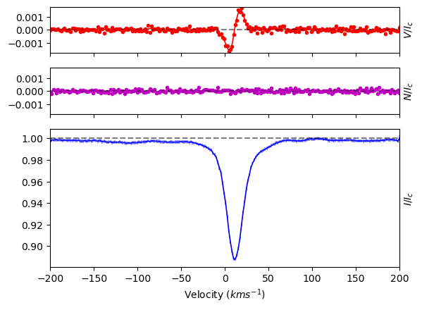
The run_lsdpy function outputs some information about the calculation. For example, it provides

the average line parameters (simple average, not SNR-weighted average),
the scaling that was used for the error bars based on the quality of the LSD model spectrum (see the next section),
an initial computation of the False Alarm Probability (FAP) and of the longitudinal magnetic field.
Warning

This automated calculation might work all right for well-behaved line profiles, but we strongly recommend that you perform a more thorough computation. See:
- From normalized spectrum to Bz measurement
- How to calculate the longitudinal field and False Alarm Probability

There is also a plot generated. If you would like to turn off the plot, simply set plotLSD=False

1.1 Setting the velocity limits/grid and the LSD weights#

In this section, we discuss some often-used options to the run_lsdpy function.

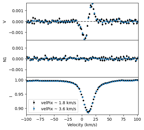
The velocity grid that is used to compute the LSD profile is controlled by the velStart, velEnd, and the velPixel keywords.

In the example above, there is a lot of continuum on each side of the profile, and we could restrict the range of velocity to, say, -100 to 100 km/s.

The default velocity step in run_lsdpy is estimated from the median pixel spacing in the observation. For ESPaDOnS spectra this is 1.8 km/s. Because the spectral line is a bit broad, we could increase this a bit to, say, 3.6 km/s and have at roughly 15 datapoints inside of the spectral line.

It’s usually good practice to set velPixel explicitly. Usually this should be set to the typical pixel size of the observation. If the lines are broad and the S/N is insufficient you could try to set the velPixel to a larger value, usually a multiple of the observation’s pixel size. Using a larger value effectively coadds pixels in the LSD process, trading resolution for higher S/N per pixel. Generally you should not set velPixel smaller than the observed pixel size. Making velPixel too small will over-sample the observation, causing artifacts in the LSD profile that look high frequency noise (clusters of single pixel spikes).

lsd2, mod2 = pol.run_lsdpy(obs=obs_file, mask=mask_file, 
                         velStart=-100.0, velEnd=100.0, velPixel=3.6, 
                         plotLSD=False)

fig, ax = lsd.plot(figsize=(5,5), label='velPix ~ 1.8 km/s')
fig, ax = lsd2.plot(fig=fig, label='velPix ~ 3.6 km/s')
ax[-1].legend(loc='lower left')
plt.show()

Another often neglected parameter that is essential to the LSD computation is the normalization weights.

The intensity (Stokes I) line weight is proportional to the line depth (\(d\)). The polarization weight (Stokes V) is proportional to \(d \times g \times \lambda\), where \(g\) is the Landé factor and \(\lambda\) is the wavelength of the line.

It is the usual practice to set these normalizing weights to a chosen ‘typical’ value. This means that the resulting LSD profile will represent a spectral line with these weights. See Kochukhov et al. (2010, A&A, 524, A5) for a complete explanation, particularly Sect. 2.5 and 2.6.

An example set of normalization values are: \(d=0.2\), \(g=1.2\), and \(\lambda=500\) nm (the default values). If you are working on a hotter or cooler star, or a different wavelength range, you may wish to chose different values.

Important

The normWave value needs to be given in nanometers

In the example below, we change the normalization depth to 0.1, the normalizing Landé factor to 1.0, and normalizing wavelength to 400 nm.

lsd3, mod3 = pol.run_lsdpy(obs=obs_file, mask=mask_file, 
                         velStart=-100.0, velEnd=100.0, velPixel=1.8,
                         normDepth=0.1, normLande=1.0, normWave=400.0,
                         plotLSD=False)

fig, ax = lsd.plot(figsize=(5,5), label='default norm.')
fig, ax = lsd3.plot(fig=fig, sameYRange=False, label='modified norm.')
ax[-1].legend(loc='lower left')
plt.show()

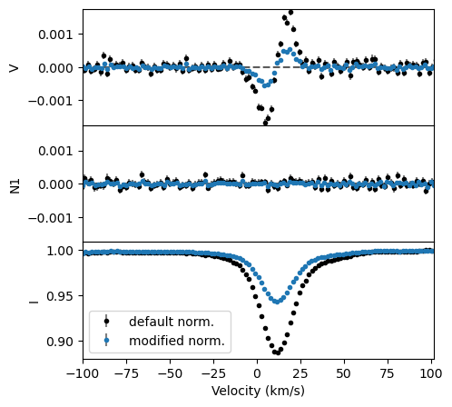
You can see that changing these parameters has a big impact on the amplitude of the LSD profile! This does not, however, change the shape of the profile. Changing the normalization parameters essentially causes the LSD profile to behave like a line with a different strength, wavelength, and Landé factor, hence the large change in amplitude of the profile.

Because these are such important parameters, they are included in the LSD object header. They will also be included in the header of the file when the LSD object is saved.

print(lsd.header)
print(lsd3.header)

# normalizing: d=0.200 lande=1.200 wl= 500.0 (I norm weight 0.200, V norm weight 120.000)

# normalizing: d=0.100 lande=1.000 wl= 400.0 (I norm weight 0.100, V norm weight  40.000)

1.2 More advanced options#

The LSDpy code and the run_lsdpy function have a set of more advanced options. For example:

The default behavior is to remove lines in the mask that are very closely spaced. Lines that are less than one LSD pixel (i.e. velPixel) apart are used for this. Weaker lines are discarded leaving only the strongest line, and line depths are combined up to a maximum of 0.6. This can very roughly approximate saturation, and it can be useful for lines that are very close due to fine or hyperfine structure. However, this behavior may not be desirable for a carefully tuned line list. This option can be turned off by setting the keyword trimMask to False.
The default behavior is to remove continuum polarization from the Stokes V LSD profile. Even with this option, large variations in the continuum polarization of the observation will still cause problems for the LSD calculation. This option can be turned off by setting the keyword removeContPol to False.
It is possible to perform a sigma clipping of the observed spectrum to reject bad pixels in the observation. This is based on a comparison between the observed spectrum and the LSD model spectrum. This option is turned off by default, but can be controlled by the sigmaClipIter and the sigmaClip keywords.

See the run_lsdpy API for more information.

2. Having a look at the model spectrum#

The run_lsdpy function also returns a Spectrum object that contains the LSD model (that is, the LSD profile convolved with the line mask – or to be more precise, it is the dot product of LSD profile vector with the mask matrix).

In the cell below, we overplot this model (purple) on the observed spectrum (grey).

spec = pol.read_spectrum(obs_file)

fig, ax = plt.subplots(2, 1, figsize=(10,8), sharex=True)
ax[1].plot(spec.wl, spec.specI, lw=2, c='0.75', label='Observation')
ax[1].set_xlim(452.0, 472.0)
ax[1].set_ylim(0.4, 1.2)
ax[1].set_xlabel('Wavelength (nm)')
ax[1].set_ylabel('Stoke I/Ic')
ax[1].plot(mod.wl, mod.specI, c='purple', lw=1, label='LSD model')

ax[0].plot(spec.wl, spec.specV, lw=2, c='0.75')
ax[0].plot(mod.wl, mod.specV, c='purple', lw=1)
ax[0].set_ylim(-0.03, 0.03)
ax[0].set_ylabel('Stokes V/Ic')

ax[1].legend(loc=0)
plt.show()

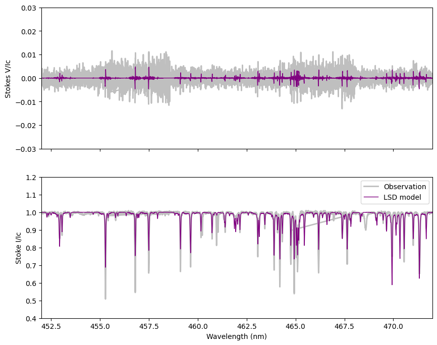
../_images/429f8a51c2c3a8ec42d08ad1ad05fd42f7ce2a202e64723874c50c218301b5c5.png

You can see that most of the lines in the observation are reproduced by the model, but there are some discrepancies. The overall fit to Stokes I is not perfect. The fit to Stokes V is better, mostly because the amplitude of the lines is smaller relative to the noise.

In the text output from LSDpy,

Modified line mask, removed 64 too closely spaced lines
Average observed spec velocity spacing: 1.810029 km/s
using a 113 point profile with 1.800000 km/s pixels
mean mask depth 0.101386 wl 494.081 Lande 1.179956 (from 1039 lines)
mean mask norm weightI 0.506930 weightV 0.480710
saving model spectrum to  ...
I reduced chi2 219.5795 (chi2 16986666.81 constraints 77473 dof 113)
 Rescaling error bars by: 14.818214
V reduced chi2 1.1248 (chi2 87017.85 constraints 77473 dof 113)
 Rescaling error bars by: 1.060586
 removing profile continuum pol: -5.5482e-06 +/- 1.2293e-08 (avg err 1.1064e-04)
N1 reduced chi2 1.1032 (chi2 85345.64 constraints 77473 dof 113)
 Rescaling error bars by: 1.050346
 removing profile continuum pol: -3.2734e-06 +/- 1.2057e-08 (avg err 1.0958e-04)
line range estimate -19.000000000000128 47.59999999999977 km/s
V in line reduced chi^2 54.634469 (chi2 2021.475344) 
 detect prob 1.000000 (fap 0.000000e+00)
 Detection! V (fap 0.000000e+00)
 V outside line reduced chi^2 1.392285 (chi2  97.459962) 
 detect prob 0.983284 (fap 1.671570e-02)
N1 in line reduced chi^2 0.952603 (chi2  35.246325) 
 detect prob 0.448573 (fap 5.514272e-01)
 Non-detection N1 (fap 5.514272e-01)
 N1 outside line reduced chi^2 1.127730 (chi2  78.941104) 
 detect prob 0.782745 (fap 2.172551e-01)

you will notice some information about the reduced \(\chi^2\) between the model spectrum and the observed spectrum.

The error bars in Stokes I and V LSD profiles are scaled up, by multiplying the formal uncertainties by the square root of the reduced \(\chi^2\). Thus LSD profiles that do a worse job fitting the observation will generally have larger uncertainties. This often leads to the Stokes I LSD profile having larger uncertainties than the Stokes V profile.

3. Saving results#

In all of the examples above, we were interested in looking at the LSD profiles produced. We did not, however, save the resulting LSD profiles nor the LSD model spectra as files!

Often we will be interested in saving the LSD profile, and perhaps the LSD model spectrum, as files straight away. The run_lsdpy function has the outLSDName and outModelName keywords to do that when it runs.

lsd, mod = pol.run_lsdpy(obs=obs_file, mask=mask_file, 
                         outLSDName='Output/prof.lsd', 
                         outModelName='Output/model.s',
                         velStart=-100.0, velEnd=100.0, velPixel=1.8, 
                         plotLSD=False)

Alternatively, you can save the results after the LSD calculation, using the save functions of the LSD and Spectrum objects.

lsd.save('Output/prof.lsd')
mod.save('Output/model.s')

Tip

Saving files can be done at anytime with the associated class functions LSD.save and Spectrum.save functions. (This is useful when manipulating LSD profiles in your workflow.)