How to use Mask objects#
In this tutorial, we go over the importance of masks and how they are made and used.
First import specpolFlow and any other packages.
What is a mask?#
Analytically, a mask is a function with Dirac deltas at wavelengths corresponding to specific spectral lines. The amplitude of the Dirac delta function corresponds to the line depth. Numerically, a mask is an array of wavelengths with a depth at the center of each line. Thus, a mask tells us the location and depth of all lines in a spectrum but does not tell us about the shape of the lines or the spectrum as a whole.
Why do we care?#
The idea behind LSD is to model a spectrum as the convolution of a line mask and a line profile (the LSD profile). So given an LSD profile and a mask, we can convolve the LSD profile with the mask to get a model spectrum. Typically, though, we have an observed spectrum and a mask but want the LSD profile. This reverse process of going from a spectrum and a line mask to an LSD profile is called deconvolution. We need a mask to help us weigh each spectral line in the spectrum so that they can be combined into an LSD profile.
Mask creation#
We will use the make_mask function to create a mask. Usually you will only need the arguments lineListFile and outMaskName, as well as two optional arguments, depthCutoff and atomsOnly.
lineListFileis the name of the file containing the line list;outMaskNameis the name of the file to write the output mask to (default is None);depthCutoffis a float that only include lines in the mask that are deeper than this value;atomsOnlyis a boolean that decides whether to include only atomic lines (no molecular lines and no H-lines).
Note
Hydrogen lines are automatically excluded when atomsOnly = True. This is done because the hydrogen lines, due to their broad wings, have a different shape than all the other lines in the spectrum.
The input line list is a VALD line list file obtained from the VALD website. It should be an “extract stellar” from VALD in their “long” format (to include Landé factors), and it should correspond to the \(T_\text{eff}\), \(\log g\), and chemical abundances of your star. More details about VALD are given in the tutorial From normalized spectrum to Bz measurement. In the example below, we start with a line list for a relatively hot star (LongList_T27000G35.dat). We use all atomic lines in the line list stronger than 0.02, except those without effective Landé factors and the H-lines.
LineList_file_name = '../GetStarted/OneObservationFlow_tutorialfiles/LongList_T27000G35.dat'
Mask_file_name = '../GetStarted/OneObservationFlow_tutorialfiles/test_output/T27000G35_depth0.02.mask'

mask_clean = pol.make_mask(LineList_file_name, outMaskName=Mask_file_name,
                           depthCutoff = 0.02, atomsOnly = True)
Warning
The make_mask function will automatically attempt to calculate the effective Landé factor for lines missing that value in the line list. It can usually make approximate estimates for lines in LS, JJ, and JK coupling schemes.
However, if a Landé factor is unable to be calculated the line will be excluded if includeNoLande = False (the default), or the Landé factor will equal the DefaultLande value if includeNoLande = True.
Mask cleaning#
After obtaining our mask, the next step is to clean it. Mask cleaning involves removing lines that we do not want to use in the computation of LSD profiles. Typically, we exclude lines that fall within the Telluric regions and those within the H line wings. The lines within the Telluric regions are contaminated by lines from Earth’s atmosphere and are therefore unusable. Hydrogen lines can’t be modelled correctly in LSD because they have a different sizes and shapes from other lines. So lines in the H wings, blended with Hydrogen lines, also can’t be modelled correctly and are unusable. Lines blended with other big broad absorption features, such as the Ca H & K lines in cooler star, should also be excluded. Although these will vary with the spectra type of the star. When dealing with stars with emission, care should be taken to exclude emission lines as they have different shapes.
This tutorial will clean the mask using some already defined regions (see How to use the ExcludeMaskRegion objects for more details). For a more detailed by hand approach see How to clean masks with the interactive tool. First we get the pre-defined telluric regions with get_telluric_regions_default and pre-defined hydrogen Balmer line regions with get_Balmer_regions_default.
# inputs
velrange = 600.0 # width of region on either side of a Balmer line to exclude, as a velocity, in km/s
# get the two sets of excluded regions and combine them
excluded_regions = pol.get_Balmer_regions_default(velrange) + pol.get_telluric_regions_default()

# optionally, display the excluded regions using Pandas
pd.DataFrame(excluded_regions.to_dict())
| start | stop | type | |
|---|---|---|---|
| 0 | 654.967529 | 657.594471 | Halpha |
| 1 | 485.167047 | 487.112953 | Hbeta |
| 2 | 433.181299 | 434.918701 | Hgamma |
| 3 | 409.349092 | 410.990908 | Hdelta |
| 4 | 396.215430 | 397.804570 | Hepsilon |
| 5 | 360.000000 | 392.000000 | Hjump |
| 6 | 587.500000 | 592.000000 | telluric |
| 7 | 627.500000 | 632.500000 | telluric |
| 8 | 684.000000 | 705.300000 | telluric |
| 9 | 717.000000 | 735.000000 | telluric |
| 10 | 757.000000 | 771.000000 | telluric |
| 11 | 790.000000 | 795.000000 | telluric |
| 12 | 809.000000 | 990.000000 | telluric |
Once we have our excluded regions, we can clean the mask using the mask.clean function. This function operates on an existing mask (it is part of the Mask class) and it takes the excluded regions. The output is a cleaned line mask, in which lines that fall within the excluded_regions have been removed. Finally we need to save the cleaned mask to a file using the mask’s save function.
# reading in the mask that we created earlier
mask = pol.read_mask('../GetStarted/OneObservationFlow_tutorialfiles/test_output/T27000G35_depth0.02.mask')

# applying the ExcludeMaskRegions that we created
mask_clean = mask.clean(excluded_regions)

# saving the new mask to a file
mask_clean.save('../GetStarted/OneObservationFlow_tutorialfiles/test_output/hd46328_test_depth0.02_clean.mask')
Other useful tools#
Interactive Line Cleaning
SpecpolFlow also includes an interactive tool to visually inspect a mask, select/deselect lines, and compare an observation with the LSD model spectrum calculated on the fly. This can be useful for fine tuning a mask. See How to clean masks with the interactive tool.
Prune
Additionally, the Mask class has a function to
prunethe mask object, removing all lines from the list that haveiuse = 0. Thecleanfunction works by setting the flagiuse = 0for lines, making them not used in a LSD calculation, but not deleting them from the line list completely. Callingpruneafter callingcleancan be used to remove the lines completely.
# using the mask that we created earlier, and re-running the clean function
mask_clean = mask.clean(excluded_regions)
print('Number of lines in the clean mask with iuse = 0: {}, from a total of: {}'.format(
    len(mask_clean[mask_clean.iuse == 0]), len(mask_clean)))

mask_clean_prune=mask_clean.prune()
print('Number of lines in the pruned mask with iuse = 0: {}, from a total of: {}'.format(
    len(mask_clean_prune[mask_clean_prune.iuse == 0]), len(mask_clean_prune)))
Number of lines in the clean mask with iuse = 0: 533, from a total of: 1601
Number of lines in the pruned mask with iuse = 0: 0, from a total of: 1068
Get Line Weights
We can calculate the LSD weight of all lines in the mask using the
get_weightsfunction. This function requires the following inputs:normDepth: the normalizing line depth, as used for LSD;normWave: the normalizing wavelength in nm;normLande: the normalizing effective Landé factor.
The function then outputs two arrays, the weights of the Stokes I lines, and the weights of the Stokes V lines. Stokes I weights are generally the line depth divided by
normDepth. Stokes V weights are (line depth * wavelength * Lande factor)/(normDepth*normWave*normLande).
weightI, weightV = mask_clean_prune.get_weights(normDepth=0.2, normWave=500.0, normLande=1.2)

print(weightI)
print(weightV)
[1.735 1.99  0.14  ... 0.25  0.285 0.335]
[1.51113292 1.52142026 0.08239234 ... 0.39070416 0.4466502  0.52675226]
Advanced mask filtering#
The Mask class supports slicing and advanced slicing like numpy. A Mask object is essentially a container for a set of numpy arrays. This means you can get a line, or range of lines, from a mask using standard syntax like mask[index_start:index_end]. This is most useful if you want to filter an existing Mask object to get only some types of lines in the mask.
# Get only lines deeper than some value
mask_deep = mask_clean_prune[mask_clean_prune.depth > 0.2]
print('total lines:', len(mask_clean_prune))
print('deep lines:', len(mask_deep))

# Get only lines in some wavelength range
mask_wl_range = mask_clean_prune[(mask_clean_prune.wl > 450.) & (mask_clean_prune.wl < 600.)]
print('mid wavelength lines:', len(mask_wl_range))

# Get only lines with larger effective Lande factors
mask_highLande = mask_clean_prune[mask_clean_prune.lande > 1.2]
print('high Lande lines:', len(mask_highLande))

# Line lists can be sliced based on element type.
# The elements codes use the format atomic number + ionization*0.01
# so they need to be rounded off before comparing numerically.
# For a line list with only iron:
mask_Fe = mask_clean_prune[np.round(mask_clean_prune.element).astype(int) == 26]
print('Fe lines:', len(mask_Fe))
# Or for a line list with no He:
mask_noHe = mask_clean_prune[np.round(mask_clean_prune.element).astype(int) != 2]
print('non-He lines:', len(mask_noHe))

# These can be combined, with numpy's logic functions.
# The parentheses are important for evaluating expressions th the right order.
# e.g. to get only strong iron lines in some wavelength range:
mask_short = mask_clean_prune[(mask_clean_prune.depth > 0.2) &
                              (mask_clean_prune.wl > 450.) & (mask_clean_prune.wl < 600.) &
                              (np.round(mask_clean_prune.element).astype(int) == 26)]
print('strong Fe lines in wavelength range:', len(mask_short))
print('wavelengths', mask_short.wl)
print('elements', mask_short.element)
print('depths', mask_short.depth)

#If you want to save the filtered mask for later use
mask_short.save('../GetStarted/OneObservationFlow_tutorialfiles/test_output/T27000G35_Fe_depth0.2.mask')
total lines: 1068
deep lines: 160
mid wavelength lines: 444
high Lande lines: 422
Fe lines: 270
non-He lines: 1024
strong Fe lines in wavelength range: 5
wavelengths [512.7371 515.6111 524.3306 583.3938 592.9685]
elements [26.02 26.02 26.02 26.02 26.02]
depths [0.21  0.263 0.25  0.262 0.213]
Plotting elements in a mask#
We can visualize the distribution of spectral lines from different chemical elements, for the whole mask or within a specific wavelength range. The plot_elementsChart function is a handy way to do this.
The plot_elementsChart function needs the arguments mask, and can use wmin and wmax to limit the wavelength range used. You can also tweak the optional arguments plotStyle, sort, and threshold.
maskis a line mask object containing the spectral line data you want to visualize.wminis a float that sets the minimum wavelength.wmaxis a float that sets the maximum wavelength.plotStyleis a string that determines the type of chart to generate. Options are'pie'or'bar'.sortis a string that controls the order in which the elements appear in the plot. You can choose:'Z'or'atomic': Sort elements by atomic number.'A'or'ascending': Sort by increasing number of lines per element.'D'or'descending': Sort by decreasing number of lines per element.
thresholdis either a float or None. It sets the minimum fractional contribution required for an element to be individually shown in the pie chart. Elements below this threshold are grouped together in an Other category. Default is None, which includes all elements.colorsis a list of colors used for the pie or bar plot.ax: an optional matplotlib axes object. If you provide one, the plot will be drawn on it. If not, a new figure and axes will be created automatically.
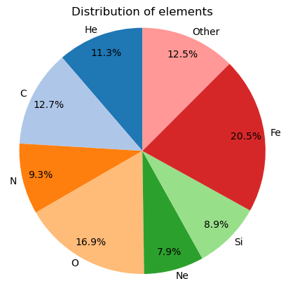
The example below shows how to plot a pie chart of the elements distribution sorted by the atomic number.
# Plot elements pie chart
pol.plot_elementsChart(mask_clean, sort='Z', threshold=0.05)
plt.show()
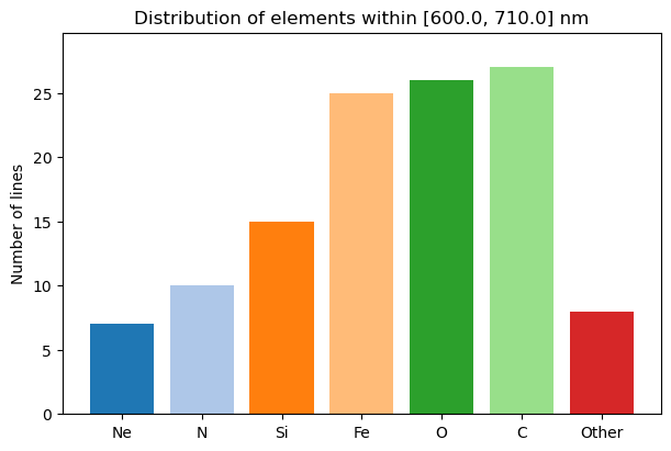
Below we illustrate how to use the bar plot with an ascending option for the sorting method. Here we only use lines between 600 and 710 nm. Note that the Other category will always be last item in the plot, regardless of the sorting method.
# Set wavelength range of lines considered
wmin = 600.0
wmax = 710.0

# Plot elements pie chart
pol.plot_elementsChart(mask_clean, wmin, wmax,plotStyle='bar', sort='A', threshold=0.05)
plt.show()
The color palette of the figure can be set by passing a list colors with the colors argument. These can be any colors matplotlib recognizes (see matplotlib’s named colors and color sequences).
The figure can be drawn into an existing matplotlib axes object by passing it with the ax argument. The plot_elementsChart function returns the figure and axes objects it used, which can be useful for making additional modifications to the figure.
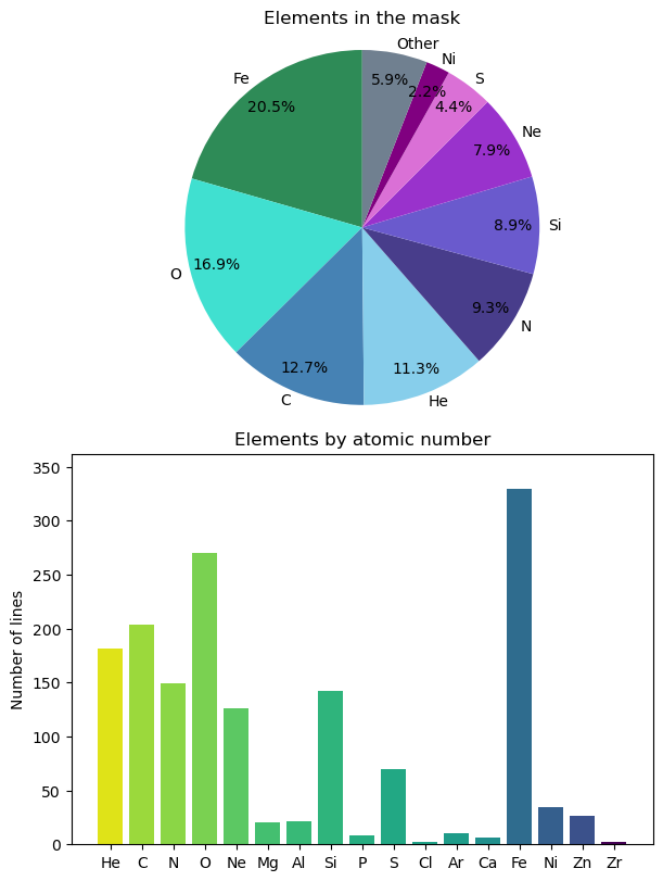
Here we illustrate a multi-panel figure with different color schemes, and change the figure titles.
import matplotlib as mpl

# Make a set of axes to draw our figures in
fig, axs = plt.subplots(2,1, layout='constrained', figsize=(6,8))
# Generate the left panel figure
fig1, ax1 = pol.plot_elementsChart(mask_clean, plotStyle='pie', sort='D', threshold=0.02, ax=axs[0],
                                   colors=['seagreen', 'turquoise', 'steelblue', 'skyblue', 'darkslateblue',
                                           'slateblue', 'darkorchid', 'orchid', 'purple', 'slategrey'])
ax1.set_title('Elements in the mask')

# Get a list of atomic numbers used in the mask
atomicNums = np.unique(np.round(mask_clean.element))
normalizedAtomicNums = atomicNums/np.max(atomicNums)

# Generate the right panel, coloring by atomic number
# (This works because we sort the bar plot by atomic number,
#  and also provide colors in order of atomic number.)
fig2, ax2 = pol.plot_elementsChart(mask_clean, plotStyle='bar', sort='Z', ax=axs[1],
                                   colors=mpl.colormaps['viridis_r'](normalizedAtomicNums))
ax2.set_title('Elements by atomic number')
plt.show()
If you have a LineList object and want to generate one of these plots for it, you can convert it to a Mask object and then use this function:
mask = pol.convert_list_to_mask(lineList, includeNoLande=True)
pol.plot_elementsChart(mask, plotStyle='pie', sort='D')
Plotting masks and using masks as line lists#
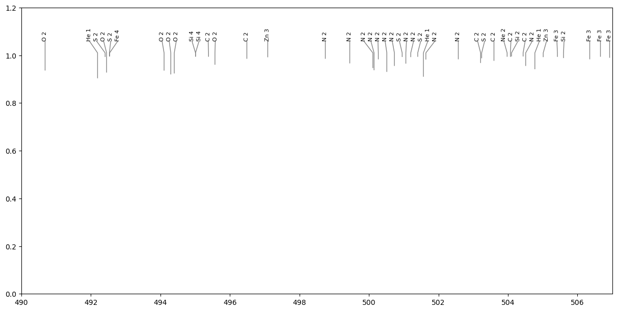
The Mask class doesn’t have a handy plotting function, but there is a plotting function for the LineList class. And the Mask class has a function for converting it to a LineList object: convert_to_line_list. The LineList object created by convert_to_line_list only contains the wavelengths, atomic species, lower level energies, effective Landé factors, and depth estimates from the mask. The other fields are left at zero, since the Mask object doesn’t contain information about them. By default convert_to_line_list will only include lines from the mask with iuse == 1.
The function plot_lineList provides options for plotting the line list (see the API docs for a variety of formatting options). Here is a basic example of how to use that, and view a portion of the Mask. The vertical ticks in this plot are proportional to the depth value in the mask.
# Convert a mask to a LineList, and then plot it
list_from_mask = mask_clean.convert_to_line_list()
fig, ax = pol.plot_lineList(list_from_mask)
ax.set_xlim(490., 507.)
plt.show()
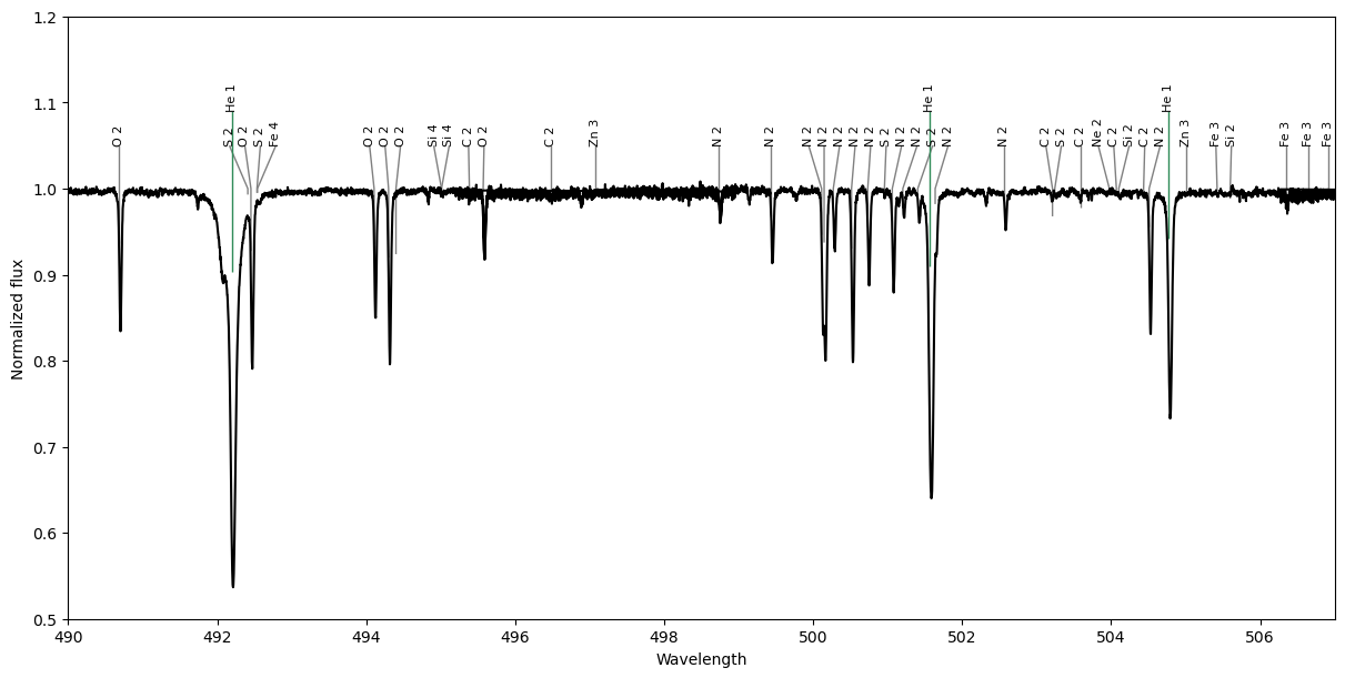
There is a convenient function for plotting sets of Spectrum objects and LineList objects: plot_obs_lines. There are some formatting options in the API docs, although plot_lineList is more flexible. This function takes a list of spectra to plot, and then a list of line lists to plot. These can be either Spectrum and LineList objects, or files that can be read as those objects.
Here we plot two line lists, made from two masks, together with the observation file hd46328_test_1.s.
# Make two masks, one containing only He lines (He I or He II), and the other with all other metal lines.
mask_He = mask_clean[(mask_clean.element == 2.0) | (mask_clean.element == 2.1)]
mask_metals = mask_clean[(mask_clean.element != 2.0) & (mask_clean.element != 2.1)]

# Convert those masks to LineList objects
lineList_He = mask_He.convert_to_line_list()
lineList_metals = mask_metals.convert_to_line_list()

# Plot an observation and those two line lists
fig, ax = pol.plot_obs_lines('../GetStarted/OneObservationFlow_tutorialfiles/hd46328_test_1.s',
                             lineList=[lineList_metals, lineList_He])
ax.set_xlim(490., 507.)
ax.set_ylim(0.5, 1.2)
plt.show()

# With the order that the LineLists are passed into the function, the one without He is the lower
# set of labels with grey ticks, while the He list is plotted above that with green ticks.
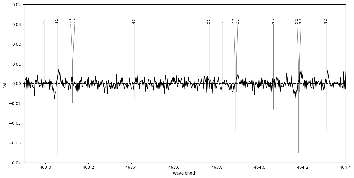
We can also use plot_obs_lines to plot Stokes V spectra. In the LSD calculation, the amplitude of the Stokes V signal is scaled by depth * lande * wavelength. Since the tickmarks are scaled by the depth parameter in the line list, we can adjust that to follow the Stokes V amplitude used by LSD.
# first we make another line list from the mask to modify
# using a mask that has had Mask.prune() called, to avoid having lines with the iuse flag = 0
list_V_plot = mask_clean_prune.convert_to_line_list()

# then we modify the depths using values from the mask
list_V_plot.depth = mask_clean_prune.depth * mask_clean_prune.lande * mask_clean_prune.wl
# and to keep the depths the right order of magnitude, we scale them by a constant
list_V_plot.depth = list_V_plot.depth/(1.2*500.)

# plot the resulting line list and the observation, using Stokes V,
# including a -12 km/s velocity (Doppler) shift for the observation
fig, ax = pol.plot_obs_lines('../GetStarted/OneObservationFlow_tutorialfiles/hd46328_test_1.s',
                             lineList=list_V_plot, velSpec=-12.0, stokes='V')
ax.set_xlim(462.9, 464.4)
ax.set_ylim(-0.04, 0.04)
plt.show()