How to Normalize Echelle Spectra with normPlot#
Introduction#
This tutorial introduces the procedure of normalizing echelle spectra with normPlot. The interactive normalization GUI is a part of the SpecpolFlow pipeline, as a step that proceeds the spectroscopic or polarimetric analysis. In this introduction to spectra normalization, we will be using ESPaDOnS observations of the star \(\xi^1\) CMa.
Note
The current version of this tutorial focuses on executing normPlot from the command line. You can also run normPlot from within a Jupyter Notebook or other Python script with
import normPlot
normPlot.normplot('[observation_file]')
Converting from the .fits format to the .s text file#
Data files downloaded from the CADC archive are distributed in a ‘.fits’ format. To use normPlot, these will need to be converted to the standard ‘.s’ text file. Note that file names ending in i.fits contain spectroscopic data (usually 4 spectra for each polarimetric observation), and file names ending in p.fits contain the spectopolarimetric data. We want to convert the p.fits files.
For this tutorial, we will use the ESPaDOns observation 2378196p.fits, so the example is specific to ESPaDOnS observations from the standard Upena/LibreESPRIT pipeline at CFHT. For observations from other instruments or other data reduction pipelines, you will need a different script to convert the FITS files to the .s format.
In the command line, write the command:
spf-fitstos-espadons 2378196p.fits
The converter will return 2378196pn.s (pipeline normalized data) and 2378196pu.s (unnormalized data) in the same directory as the ‘.fits’ file.
Normalization GUI#
Our goal is to fit a low order polynomial through “good” continuum points in every spectral order. The continuum can then be normalized by dividing the observation by the fit. This creates a “common line” (a flat horizontal line at y = 1) which can be used to consistently measure the properties of the spectral lines.
Note
normPlot is an optional extra, and is not installed by default with specpolFlow. If you have not used the option to install it, you can install it now with
pip install normPlot
Open the normalization GUI from the command line with
normplot <observation_file.s>
This generates a new window with the spectrum separated into orders, which are indicated by different colors. Also shown are polynomial curves, which are fits to the continuum for each order, colored differently for each order. The black points are the points the used to generate the polynomial fit.
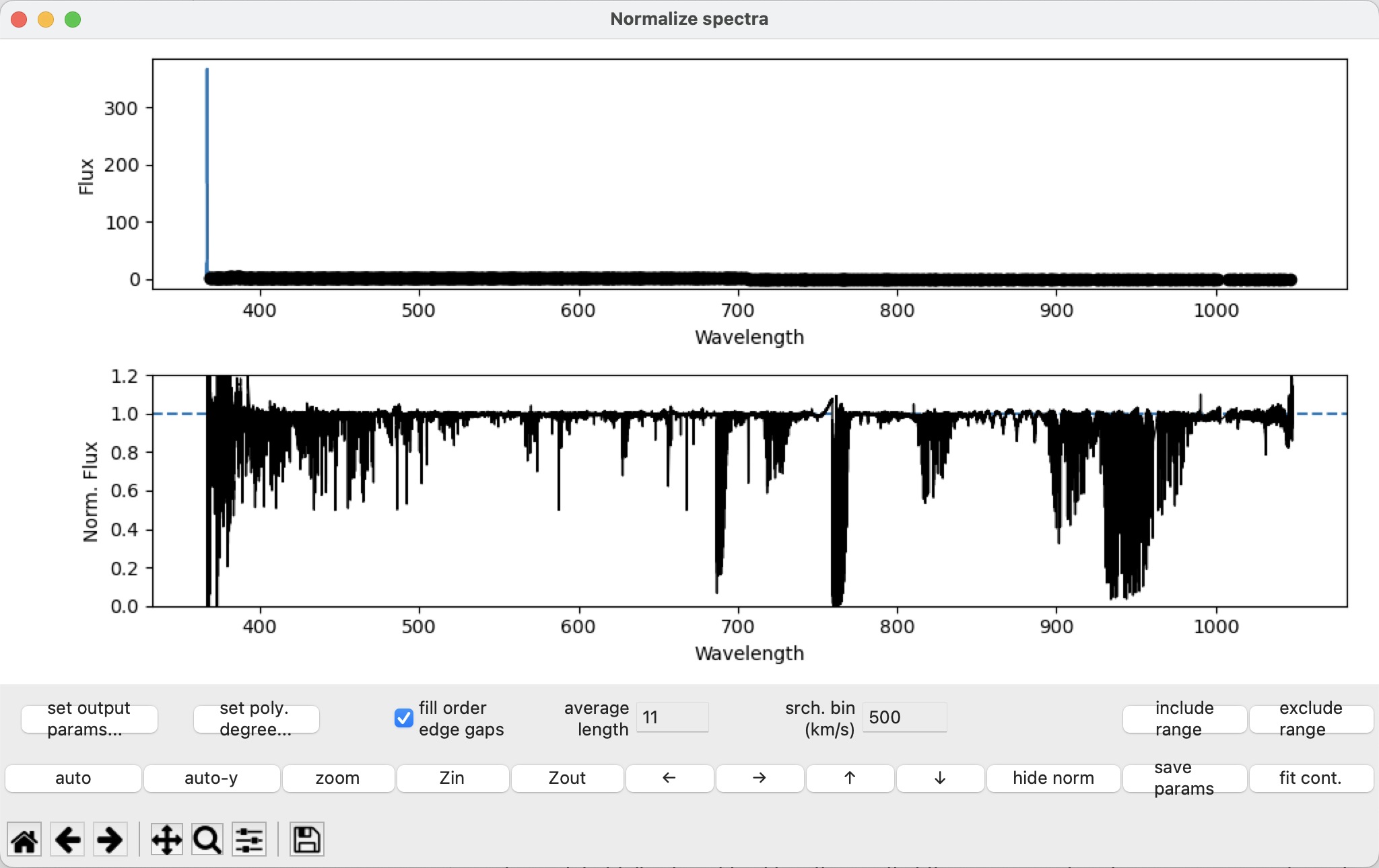
The bottom left corner of the window contains a toolbar with commands from matplotlib (panning, zooming, returning to default, saving a figure). Above that are a set of buttons with some custom commands for automatically scaling both axes, auto-scaling just the y-axis, zooming, and panning. There are keyboard shortcuts for these commands (arrow keys for panning, ‘a’ for auto-scaling, ‘A’ for auto-scaling the y-axis, ‘z’ for zooming on a selected region, ‘i’ and ‘o’ for zooming in and out).
The fit points#
We want to select a relatively small number of “good” continuum points that can be used for a polynomial fit describing the continuum of the observation. These “good” points, which appear as black dots on the plot, are selected within an order and are used to fit a polynomial function for the continuum for that order. Ideally, the resulting normalized continuum will be equal to 1.
To find “good” points, each order is broken down into a set of consecutive search bins in wavelength. The bins are equal in width (in velocity). In each bin, the highest flux point is selected as being most likely in the continuum (i.e. not in an absorption line). However, to deal with noise in the observation, a running average is applied to the spectrum before selecting the highest point in the search bin. This averaging helps ensure that the selected highest point in a bin is not highest because of a peak in the noise, but instead highest because of real features in the spectrum.
Normalizing the individual orders#
normPlot normalizes each spectral order individually. It calculates a separate best fit polynomial for each order, and divides each observed order by that order’s polynomial. Because of this, it is useful to look through the fit to the observation, paying attention to one order at a time, when trying to optimize the normalization.
Setting global fitting parameters#
There are two parameters that apply to all the spectral orders: the srch. bin (km/s) value and the average length value.
The srch. bin (km/s) value controls the size of the bin used to find a “good” continuum point. This should be set large enough so that there is some real continuum inside most bins. This should be at least several times larger than the \(v\sin i\) of the star. If \(v\sin i\) is very high, or if line blending is severe in the observation you may want a larger srch. bin than the default value. On the other hand if \(v\sin i\) is low and there is not much blending you can use a lower value than the default.
If normPlot is selecting points (black circles in the plot) inside lines, that is usually a sign that you should increase the srch. bin value. This is usually a problem on the blue end of an observation where the line density is highest.
In this tutorial we use the default 500 km s\(^{-1}\) search bin width. The example \(\xi^1\) CMa is a B-type star and so line blending isn’t too bad.
The average length value controls the running average used before finding the “best” (highest) point in a bin. This is used to reduce the impact of noise on the selected “good” points. The default value is ok for observations with quite high S/N, but for noisier observations a larger value is better. If the selected “good” points are sitting a little above the center of the noise distribution (in continuum regions), that’s usually a sign you should increase the average length. In this tutorial we use the default 11 pixel average length, since the S/N of the observation is quite good.
Telluric or noise dominated orders#
In some instances, the observations may have orders that have very low signal to noise ratios, or which are dominated by telluric lines (sharp lines created from absorption by Earth’s atmosphere). It can be difficult to try to apply the full set of fitting procedures on these orders to get them flat. Moreover, these orders contain very little useful information about the real spectrum of the star.
In these cases, it can be more expedient to simply achieve a reasonably well-behaved continuum polynomial fit, rather than doing a detailed normalization for the problem order. You can try reducing the order of the polynomial degree by clicking the set poly. degree... button. For our example, change orders 1, 2, 38, 39, 40 to have smaller values (like 1 or 2).
Removing spectral lines from the fit#
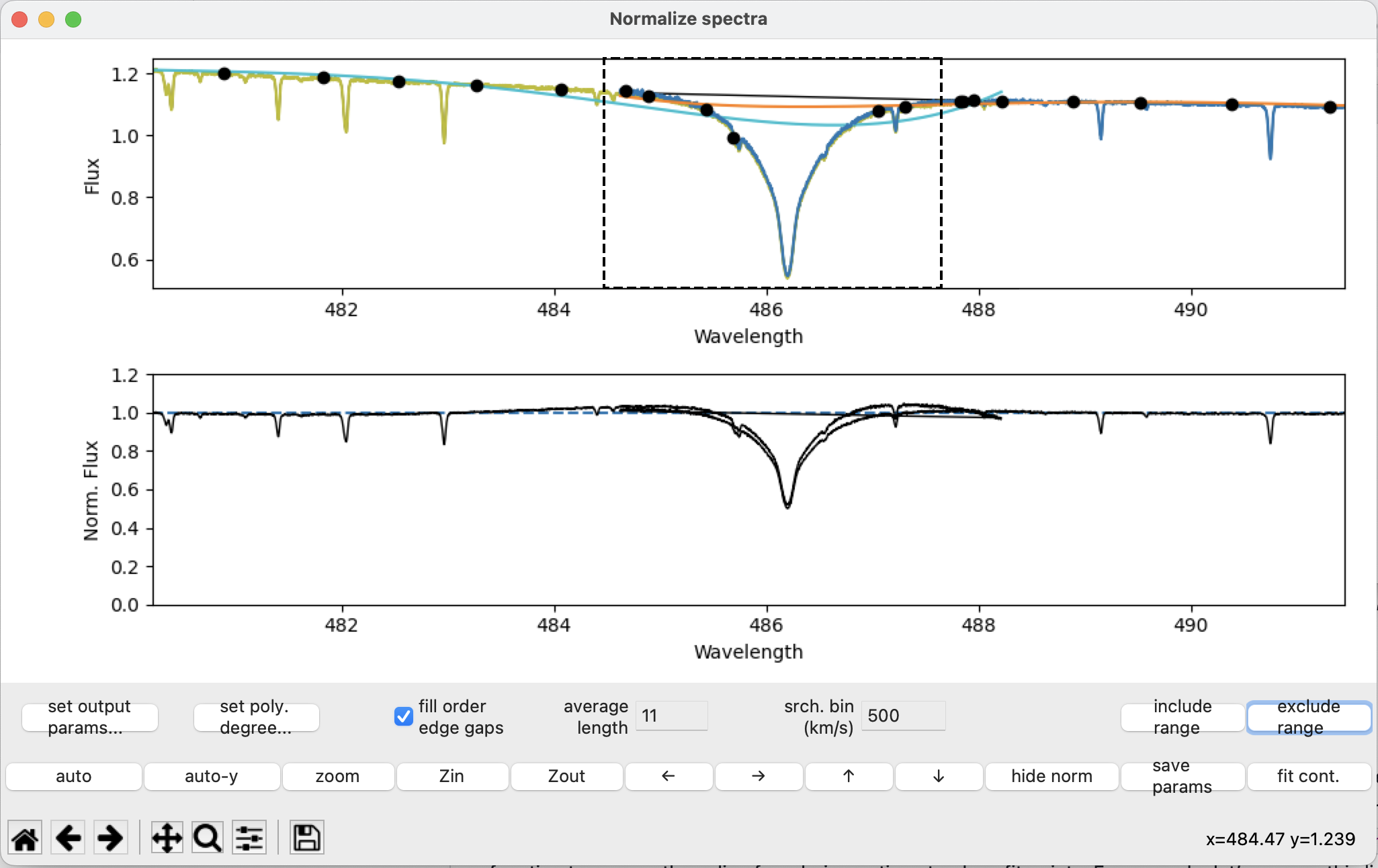
It is important to make sure that spectral lines are not contributing to the polynomial fit. None of the “good” continuum points should appear within spectral lines. Use the exclude range function to remove points within spectral lines from the fit. For example, let’s remove the \(H \beta\) line at ~486 nm.
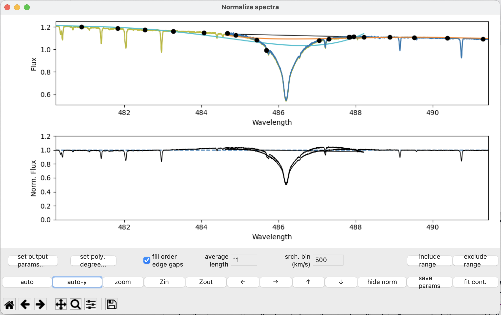
Select the region using the exclude range button:
After pressing fit cont:
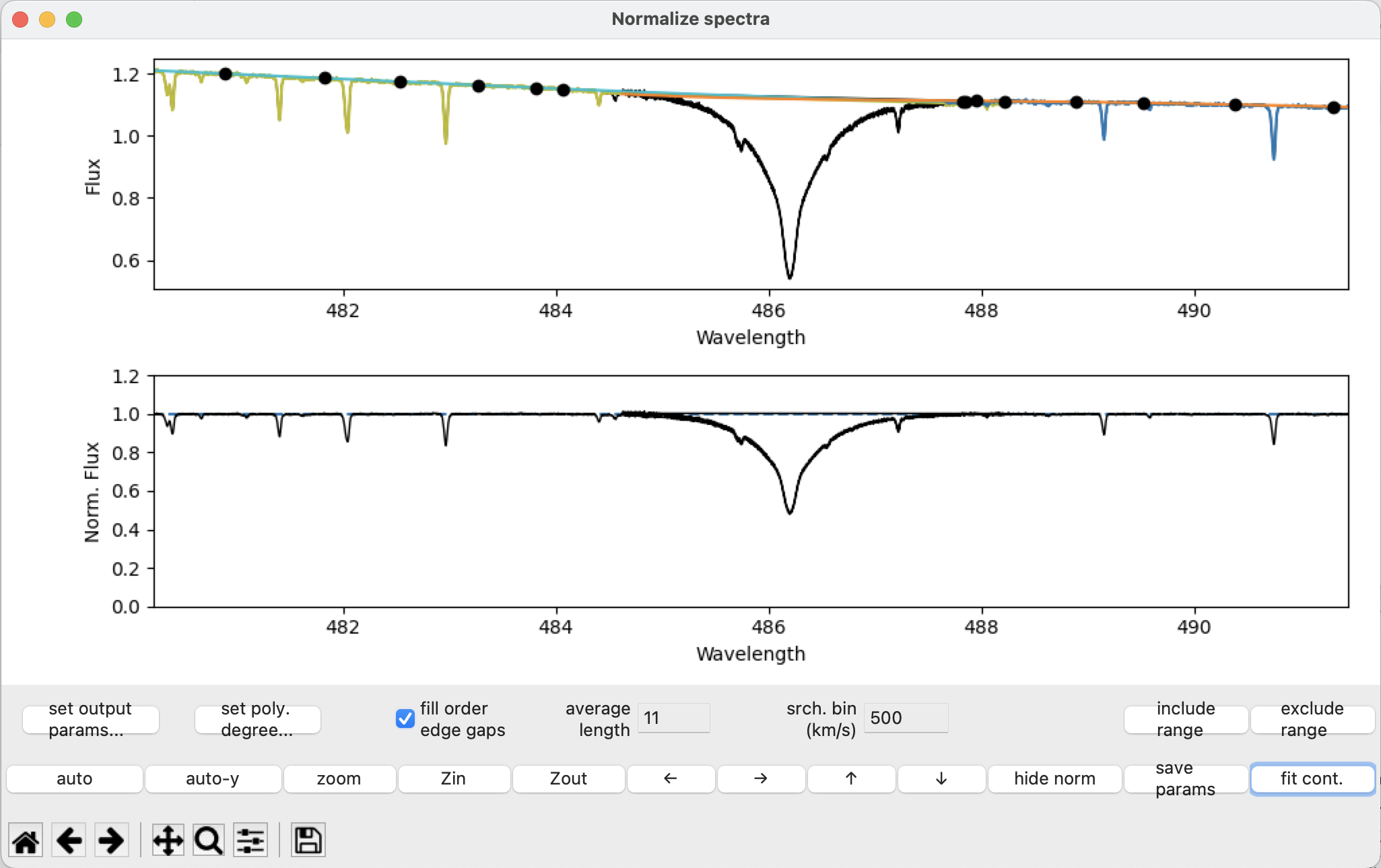
The wings of the \(H \beta\) line should no longer be arching above the continuum since we excluded the problem points from the fitting routine!
If your exclude region is too big, you can use the include range button to bring useful portions of the spectrum back into the fit.
Now, try removing the big broad spectral lines at the following wavelengths: 383, 397, 410 (\(H \delta\)), 434 (\(H \gamma\)), 438, 447, 656 (\(H \alpha\)), 855, 860, 866, 875, 886, 901, and 905 nm.
If we adjust the width of the search bins later, we will not have to worry about new points appearing inside these lines, since we have removed them.
In some instances, we will have spectral lines that exist on the overlapping edge of two orders like \(H \alpha\) and \(H \beta\). For some lines, this can be managed by having the fill order edge gaps option turned on (it defaults to on). Then, for that excluded region, the program use the nearest “good” fit point from the neighboring order to constrain the polynomial for this order. If the fluxes from different orders agree well (the flat fielding and blaze correction are good) this is helpful. If the blaze correction is particularly bad you may want to turn this off.
When you have removed a large part of an order from the fit, the polynomial may have too high a degree for the remaining part of the order. This problem is most common in Balmer lines and other very wide features. It mostly shows up as the fit polynomial curving too much inside the region that has been excluded. Here is an example of that around \(H\delta\):
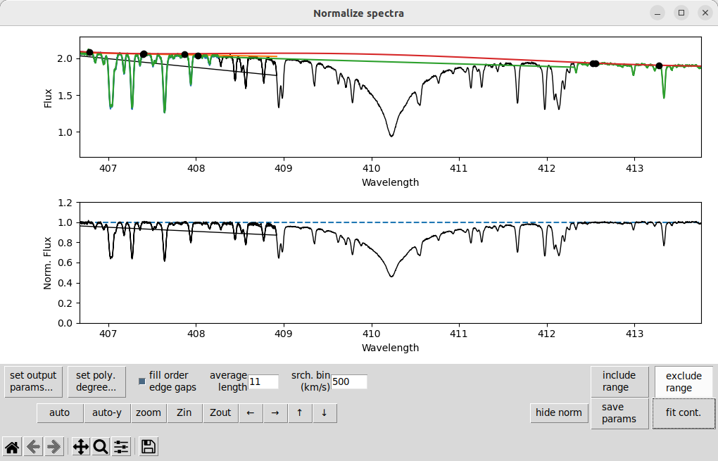
The solution is usually to decrease the degree of the polynomial, click set poly. degree..., go to order 7 (for this example), and change the polynomial degree to 3. Then after pressing fit cont we get:
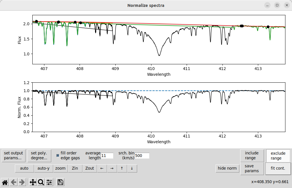
That is a bit more reasonable. If this were an A-type star with even broader Balmer lines you might need to reduce the degree to 2 or even 1!
Fit points in telluric lines#
You may occasionally find some fit points being placed inside telluric lines. This usually only happens in places where a lot of telluric lines blend together, so that there is no good continuum in a region of spectrum. We exclude those regions, again with the exclude range button. For example let’s exclude the region around 759 nm.
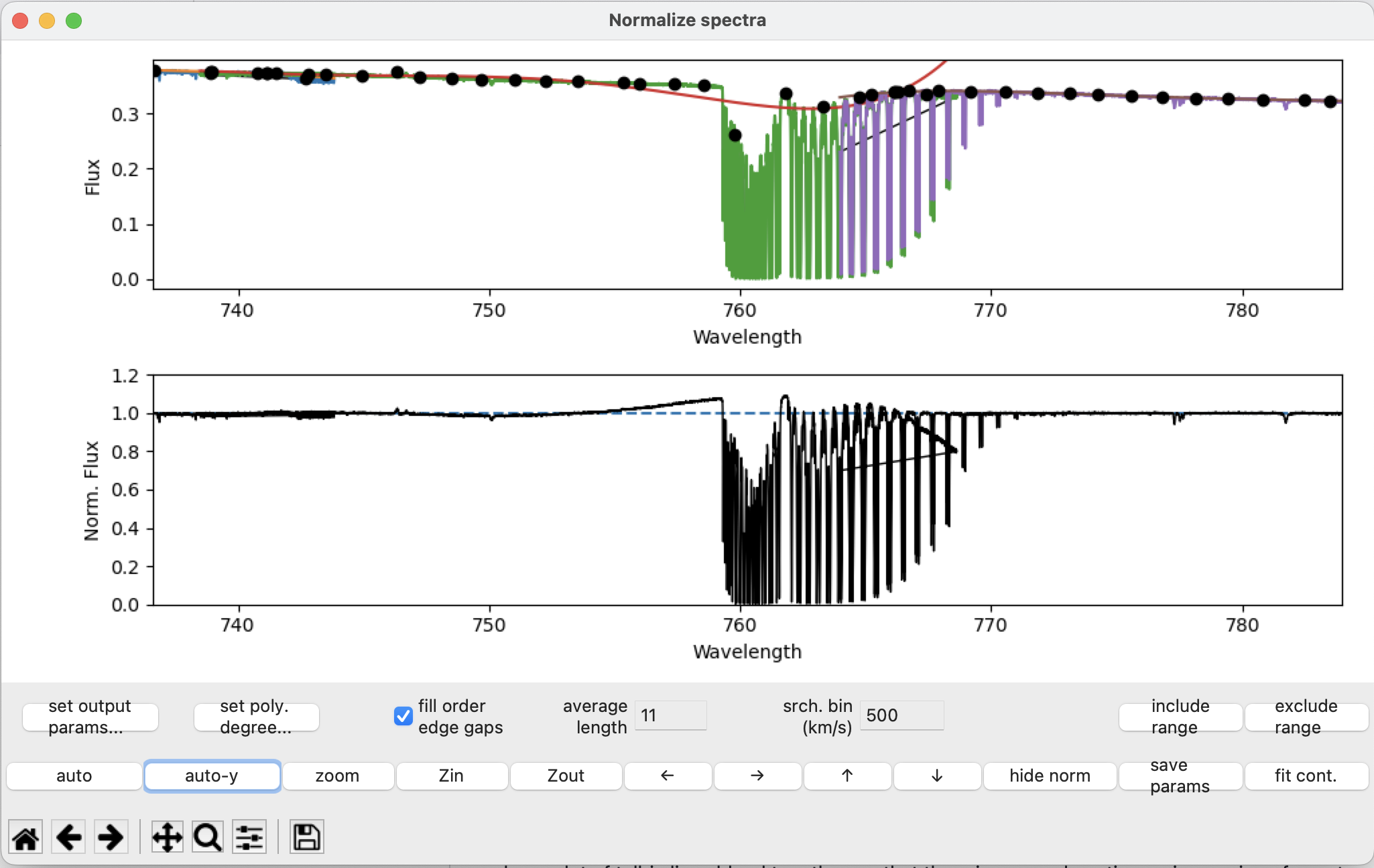
Select the region using the exclude range button, then after pressing fit cont:
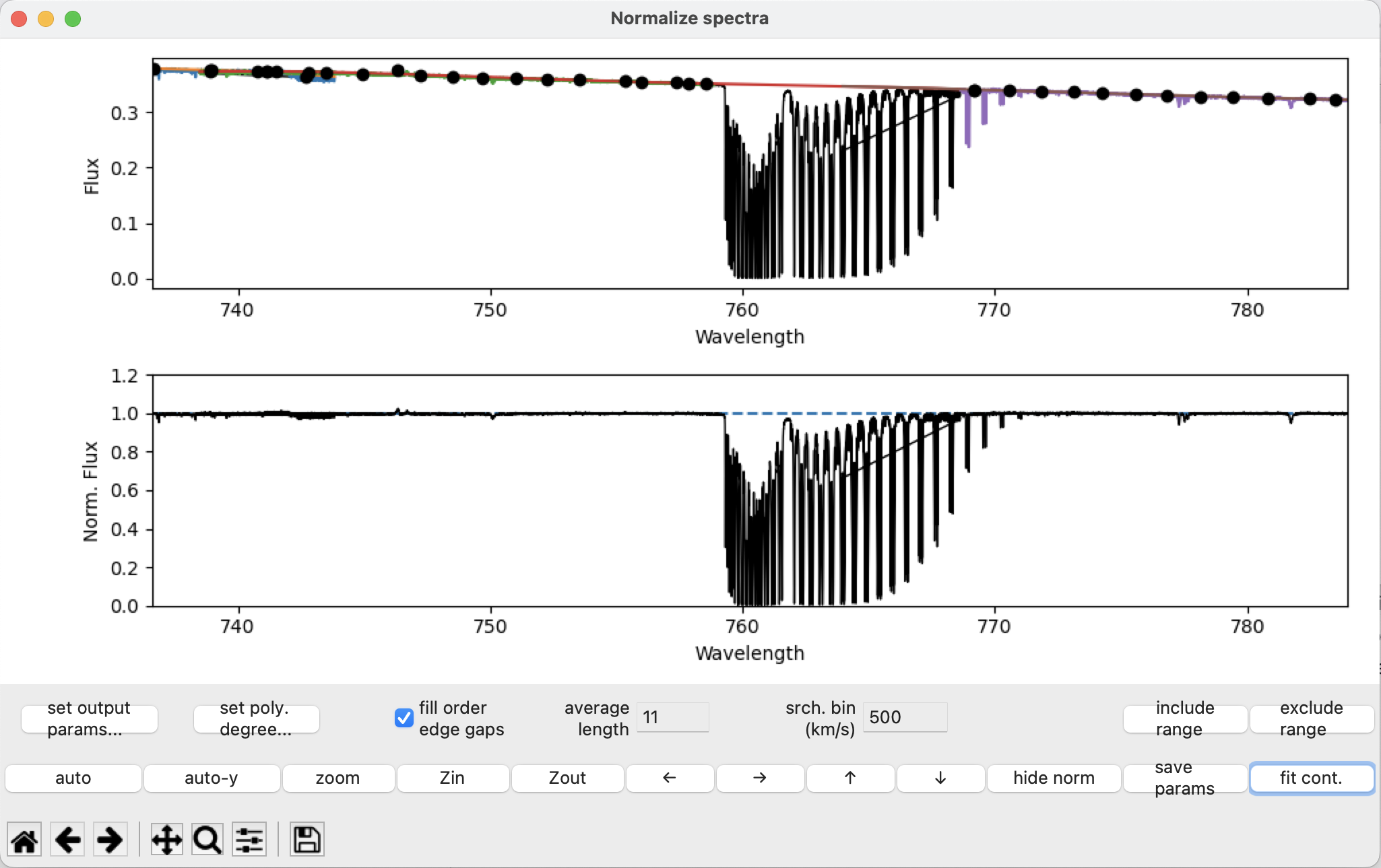
The continuum near the telluric region around 759 nm is no longer arched, and there are no fit points within the blended region.
Removing emission lines#
There are a few weak emission lines in this spectrum. In the case of \(\xi^1\) CMa, the emission lines are pretty weak and could almost be ignored. But in a star with more emission, this will cause problems. Emission lines don’t work with the algorithm normPlot uses for selecting “good” points: if the emission line makes the highest point in a bin, it will be selected, even though it is definitely not continuum! To solve this you need to remove emission lines using the exclude range button. Really strong cosmic ray hits may cause a similar problem, so if they are being selected as “good” points they should also be removed.
Here is an example of a weak emission feature at about 672 nm that is throwing off a polynomial fit:
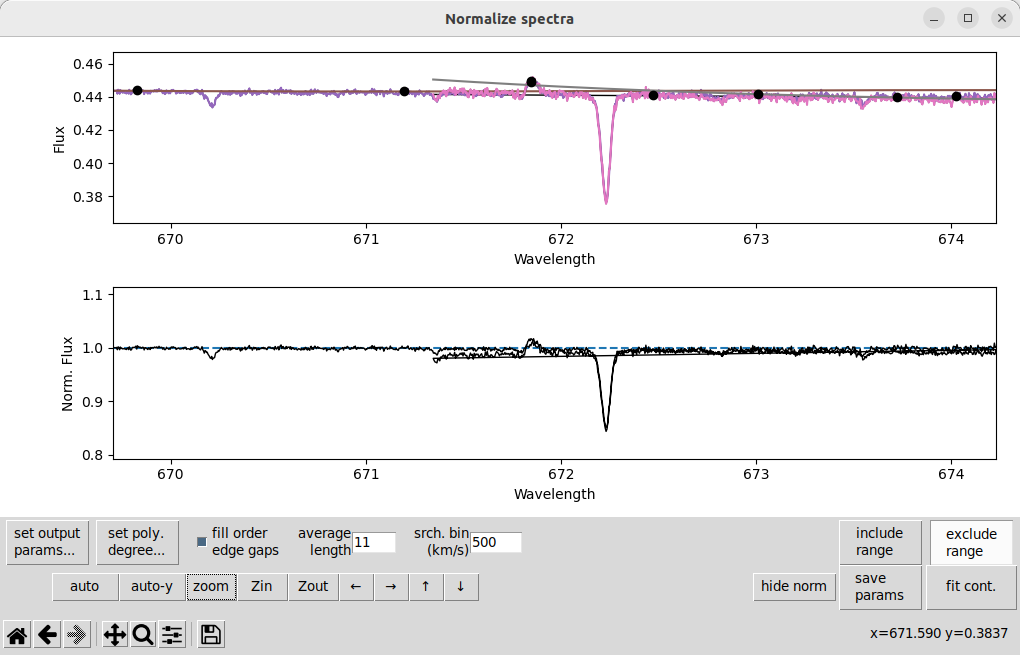
In this case, it is causing some extra trouble because it is at the very edge of one spectral order (you can see the overlapping orders here). When we remove this line using the the exclude range button, then use fit cont, we get:
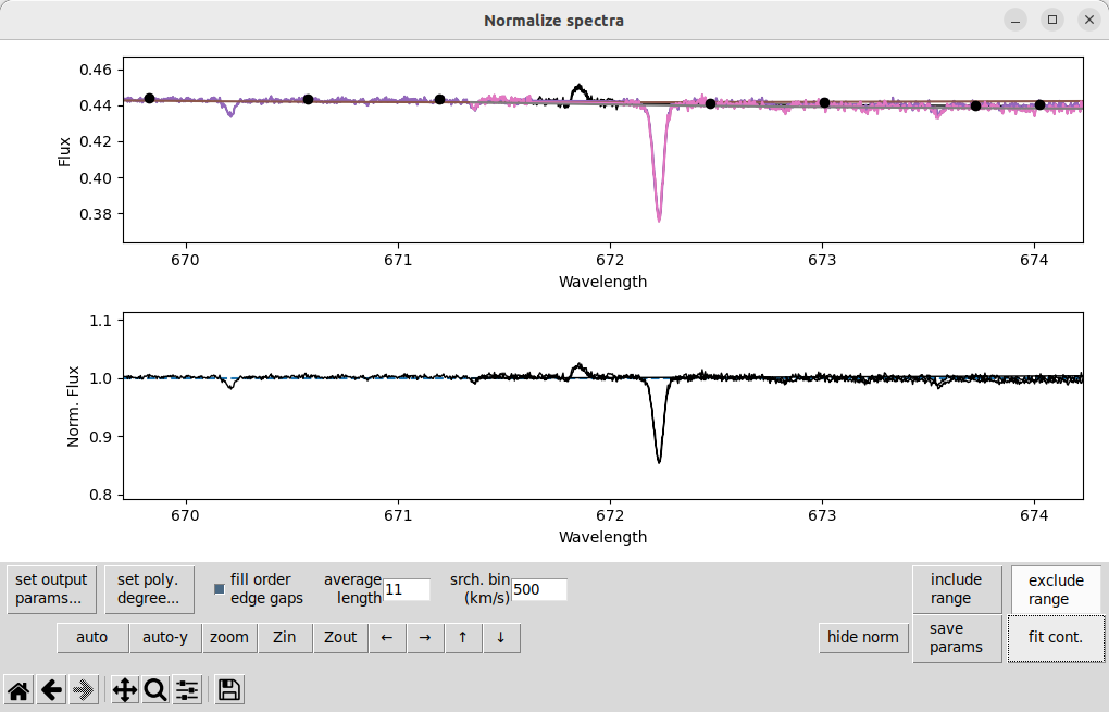
That solves the problem nicely. Some other weak emission features that should be removed in this observation are at 646, 746, 810, and 990 nm.
Fit Points on Noise#
You may occasionally find a “good” fit point resting too high in the noise on the continuum. This is mostly a problem for spectra with more noise. To correct this, adjust the average length and increase it to a slightly larger number. (In situations where noise is very important you may need to double or triple the value.)
For computing the “good” points, there is a small window of width that we specify (in pixels). For each data point in the spectrum, an average flux is calculated using the pixels within that window, centered on the data point we care about. This creates a moving average, which moves across the spectrum one data point at a time. Adjusting the average length essentially smooths the spectrum contained in that bin. This applies to the selected “good” points for the polynomial fit, but does not directly affect the data in the normalized spectrum. In effect, this will decrease the impact of the noise on where the fit points are placed.
Saving normalized spectra#
Closing the main window always automatically saves the normalized spectrum. However, it is a good idea to push the fit cont. button before closing the program. The program uses the current polynomials without updating them for any changes when it is closed, so it is a good idea to make sure they are up to date with your final parameters.
The chosen fitting parameters (after fitting) can be saved using the save params button to the files: exclude.dat, poly-deg.dat, and params.dat. These files can later be loaded to start from where you left off, or for a good initial guess if you are normalizing similar spectra. Usually it’s safest to always click this button before closing the main window, just in case you want to tweak a normalization later.
Output files#
Once the main window is closed the program will save the normalized spectrum to [observation_file].norm.
Note
The output will use the normalization and parameters of the last update. It is advised that you use the fit cont. button before closing the window.
If you clicked the save params, the program will also write out the fitting information in the files exclude.dat, poly-deg.dat, and params.dat. When you are satisfied with the normalization, it is useful to make a copy of these files with a name unique to the data.
Running normPlot with previous parameters#
When running normPlot again, it will check for the parameter files and try to read them if they exist: exclude.dat, poly-deg.dat, and params.dat. Alternatively, you can run normPlot using copies of those files with specified names from the command line:
normplot -e [exclude_file] -d [poly-deg_file] -c [params_file] [observation_file]
or within Python:
import normPlot
normPlot.normplot('[observation_file]',
                  excludeRegionName='[exclude_file]',
                  polynomialsName='[poly-deg_file]',
                  paramsName='[params_file]')
You can also take the parameter files and apply them to spectra without having the reopen the interface. This uses the -b flag from the command line:
normplot -b -e [exclude_file] -d [poly-deg_file] -c [params_file] [observation_file]
or the batchMode=True argument in Python:
normPlot.normplot('[observation_file]',
                  excludeRegionName='[exclude_file]',
                  polynomialsName='[poly-deg_file]',
                  paramsName='[params_file]',
                  batchMode=True)
This useful for normalizing a large number of observations of the same star.
