How analyze individual spectral lines

Many of the tools in SpecpolFlow can be applied to a single line in an observed spectrum. In this example we analyze a few emission lines in the spectrum of a T Tauri star.

First, import SpecpolFlow and some packages that will help with data visualization.

import specpolFlow as pol

import pandas as pd
import matplotlib.pyplot as plt

1. Create individual line file

In this tutorial, we use the UPENA normalized spectrum (IndividualLine_tutorialfiles/1423137pn.s) of the active cool star BP Tau.

We first load in the spectrum.

spec = pol.read_spectrum("IndividualLine_tutorialfiles/1423137pn.s")

To create extract an individual line from the spectrum, we have to define the transition wavelength lambda0 and a range with respect to the line center. In the example below, we select the HeI line at 667.815 nm in a 0.6 nm window.

# Create individual line profile 
lambda0 = 667.815 # He i 667.815 nm
geff = 1.0 # He i 667.815 nm, used later for calculating Bz
lwidth = 0.3 

prof = spec.individual_line(lambda0 = lambda0, lwidth = lwidth)

The individual_line function returns prof, which is really an LSD profile object, and inherits all the attributes from the LSD class. Therefore, you can use all the functionality discussed in the LSD Class Tutorial (i.e., one can normalize, slice, or shift the line profile).

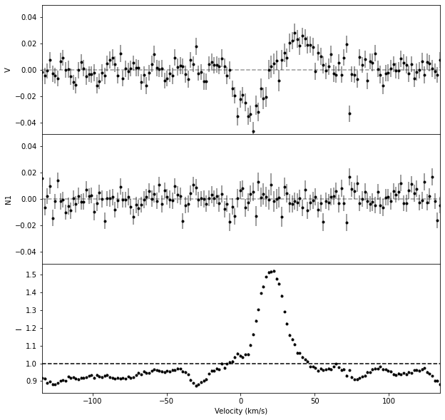
Below, we visualize the individual line using the plot class function.

fig, axes = prof.plot()
axes[-1].axhline(1, color ='k', ls = '--')

<matplotlib.lines.Line2D at 0x7f040b391a50>

2. Calculate Bz

To calculate the longitudinal field (Bz) of the individual line, we can use the calc_bz function of the LSD class.

# Define the limits for the continuum normalization
cmin = -50.0; cmax = 80.0

# Compute Bz in a 45 km/s window
Bz, fig = prof.calc_bz(norm = 'auto', cog = 'I', 
                   velrange = [cmin, cmax], bzwidth = 45.0, 
                   geff = geff, lambda0 = lambda0,
                   plot = True)

using AUTO method for the normalization
  using the median of the continuum outside of the line

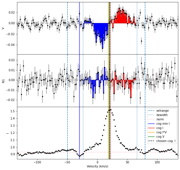
We can then display the results using the pandas dataframe. For this particular line, we find Bz \(= 1.2 \pm 0.1\) kG.

Bz_df = pd.DataFrame(data = [Bz])

# Simple display of the pandas dataframe
Bz_df.style

	V bz (G)	V bz sig (G)	V FAP	N1 bz (G)	N1 bz sig (G)	N1 FAP	N2 bz (G)	N2 bz sig (G)	N2 FAP	norm_method	norm	cog_method	cog	int. range start	int. range end
0	1191.652271	130.184898	0.000000	-34.686996	130.041356	0.564259	0.000000	0.000000	0.000000	auto	0.931285	I	21.173209	-23.826791	66.173209

3. Normalize the individual line

In the figure above, we see that calc_bz improved the continuum normalization, taking the median of the continuum outside of the line. Therefore, we propagate this normalization in the prof object before saving the individual line profile into a file.

# Renormalize prof using the continuum value obtained by calc_bz
prof_norm = prof.norm(Bz['norm'])

# Display the profile
fig, axes = prof_norm.plot()
axes[-1].axhline(1, color = 'k', ls = '--')

<matplotlib.lines.Line2D at 0x7f0401fed2a0>

4. Saving individual lines

Finally, you can save the individual line into a file using the save function, shown below. This file will have a text format like an LSD profile.

prof_norm.save("Output/1423137.Helium")

5. Dealing with order overlaps

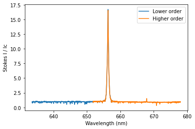
Now, let’s do the same for the Halpha line. However, there is a complication, the Halpha line is split across two orders in this echelle spectrum.

# reading the spectrum
spec = pol.read_spectrum("IndividualLine_tutorialfiles/1423137pn.s")
# defining the line parameters
lambda0 = 656.281 ;  geff = 1.0 # Halpha
lwidth = 700. * lambda0 / 2.99e5 #convert a 700 km/s width into a width in nm
# getting the profile for that line
prof = spec.individual_line(lambda0 = lambda0, lwidth = lwidth)

# Define the limits for the continuum normalization
# Compute Bz in a 200 km/s window around the cog
cogRange = [-400., 400.]
intRange = 200.
Bz, fig = prof.calc_bz(norm = 'auto', cog = 'I', 
                       velrange = cogRange, bzwidth = intRange, 
                       geff = geff, lambda0 = lambda0,
                       plot = True)   

# Create a dataframe to record the result of the different methods in this section
d = {'Merge type':'None'}
d.update(Bz)
df_results = pd.DataFrame(data = [d])
df_results.style

using AUTO method for the normalization
  using the median of the continuum outside of the line

/tmp/ipykernel_980312/871814974.py:13: UserWarning: 
 The velocity array is not monotonically increasing. 
 There might be an order overlap in the region of the observation used. 
 calc_bz will sort the LSD profile in velocity order. 
 Make sure this is what you want -- merge orders before running calc_bz()!
  Bz, fig = prof.calc_bz(norm = 'auto', cog = 'I',

	Merge type	V bz (G)	V bz sig (G)	V FAP	N1 bz (G)	N1 bz sig (G)	N1 FAP	N2 bz (G)	N2 bz sig (G)	N2 FAP	norm_method	norm	cog_method	cog	int. range start	int. range end
0	None	72.964936	17.843167	0.000000	7.405907	17.843162	0.435065	0.000000	0.000000	0.000000	auto	1.101100	I	9.725353	-190.274647	209.725353

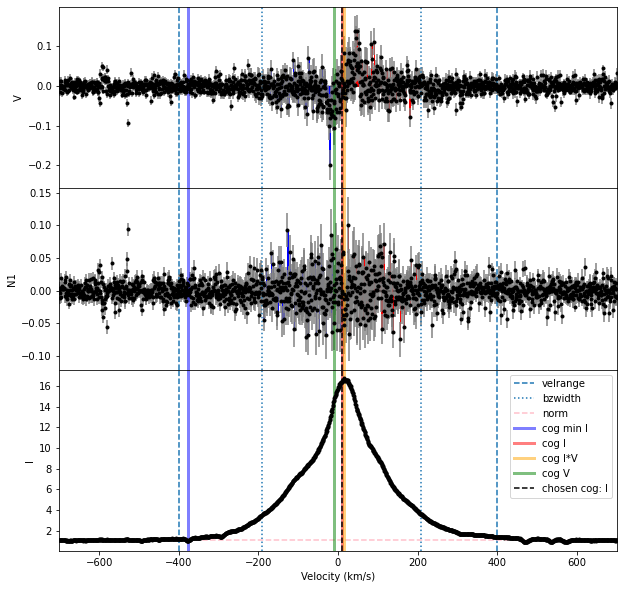
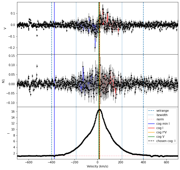
The calc_bz function gave us a warning about there probably being different spectral orders here. And the plot of results is relatively messy.

5.1 Option 1: Selecting only one order

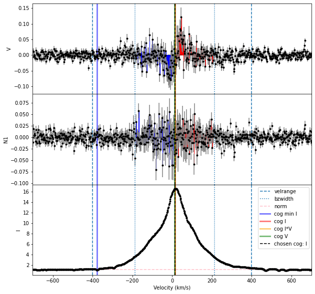
The simplest solution to this problem is to only use one spectral order for the Bz calculation. In the case of this Halpha line, both orders include the center of the line that we are interested in. So we can calculate Bz from the two orders separately.

To get the spectral orders that include a wavelength, or range of wavelengths, we can use the get_orders_in_range function of the Spectrum class. This returns a list containing Spectrum objects for each order.

## Selecting only one order
orders = spec.get_orders_in_range(lambda0)
print('There are {} orders with Halpha in them'.format(len(orders)))

# Illustration of the order overlap
fig, ax = plt.subplots(1,1)
ax.plot(orders[0].wl, orders[0].specI, label = 'Lower order')
ax.plot(orders[1].wl, orders[1].specI, label = 'Higher order')
ax.set_xlabel('Wavelength (nm)')
ax.set_ylabel('Stokes I / Ic')
ax.legend(loc = 0)

# loop over the orders
type = ['lower only', 'higher only']
i = 0
for ord in orders:

    # get the profile for the line in this order
    prof = ord.individual_line(lambda0 = lambda0, lwidth = lwidth)

    # compute Bz, in the defined velocity window around the cog
    Bz, fig = prof.calc_bz(norm = 'auto', cog = 'I', 
                           velrange = cogRange, bzwidth = intRange, 
                           geff = geff, lambda0 = lambda0,
                           plot = True)
    d = {'Merge type':type[i]}
    d.update(Bz)
    df = pd.DataFrame(data=[d])
    df_results = pd.concat([df_results,df], ignore_index=True)
    i += 1

# display the Bz result as a dataframe
df_results.style

There are 2 orders with Halpha in them
using AUTO method for the normalization
  using the median of the continuum outside of the line
using AUTO method for the normalization
  using the median of the continuum outside of the line

	Merge type	V bz (G)	V bz sig (G)	V FAP	N1 bz (G)	N1 bz sig (G)	N1 FAP	N2 bz (G)	N2 bz sig (G)	N2 FAP	norm_method	norm	cog_method	cog	int. range start	int. range end
0	None	72.964936	17.843167	0.000000	7.405907	17.843162	0.435065	0.000000	0.000000	0.000000	auto	1.101100	I	9.725353	-190.274647	209.725353
1	lower only	94.012588	25.428151	0.000003	5.209152	25.428140	0.221315	0.000000	0.000000	0.000000	auto	1.104800	I	14.197130	-185.802870	214.197130
2	higher only	54.213318	21.662775	0.000007	3.435552	21.662771	0.803308	0.000000	0.000000	0.000000	auto	1.096300	I	13.943177	-186.056823	213.943177

5.2 Option 2: merging the orders

An alternative solution is to merge the spectral orders before calculating Bz. Combining orders is more complex, but it can optimize S/N, and it can be useful when the wavelength range of interest extends beyond the edge of an order.

We can combine spectral orders with the merge_orders function of the Spectrum class. This function provides two methods of combining orders 'trim' and 'coadd'. This function only really works properly if the continuum levels are consistent between orders.

In merge_orders with mode = 'trim', the function just uses the first order up to the midpoint of the region where the orders overlap, then it uses the second order beyond that midpoint. This approach is relatively simple and essentially throws away a bit of signal. But it is more robust against errors in continuum normalization (or spectrum extraction) at the edges of spectral orders, and these errors are relatively common.

In merge_orders with mode = 'coadd', the function essentially averages the orders, weighted by the uncertainties on individual pixels (specifically by \(1/\sigma^2\)). To do this it needs to interpolate in wavelength, and it uses the wavelengths from the first order, interpolating the second order onto that grid. This mode requires reliable uncertainties for the Stokes I spectrum. This approach has the advantage that it optimizes the S/N in the merged spectrum. But it is more vulnerable to continuum normalization errors at the edges of orders, since an error in either order will cause problems for the merged result.

Here we try out both methods to compare the results. In this case the normalization is pretty good in the region we care about, so the 'coadd' mode gives a more precise result.

## Merging using the trim method
merge = spec.merge_orders(mode = 'trim', midpoint = 0.5)

prof = merge.individual_line(lambda0 = lambda0, lwidth = lwidth)
Bz, fig = prof.calc_bz(norm = 'auto', cog = 'I', 
                       velrange = cogRange, bzwidth = intRange, 
                       geff = geff, lambda0 = lambda0,
                       plot = True)
d = {'Merge type':'trim at mid-point'}
d.update(Bz)
df = pd.DataFrame(data = [d])
df_results = pd.concat([df_results,df], ignore_index=True)


## Merging using the coadd method
merge = spec.merge_orders(mode='coadd')

prof = merge.individual_line(lambda0 = lambda0, lwidth = lwidth)
Bz, fig = prof.calc_bz(norm = 'auto', cog = 'I', 
                       velrange = cogRange, bzwidth = intRange, 
                       geff = geff, lambda0 = lambda0,
                       plot = True)
d = {'Merge type':'coadd'}
d.update(Bz)
df = pd.DataFrame(data = [d])
df_results = pd.concat([df_results,df], ignore_index = True)

# Display the Bz result as a dataframe
df_results.style

using AUTO method for the normalization
  using the median of the continuum outside of the line
using AUTO method for the normalization
  using the median of the continuum outside of the line

	Merge type	V bz (G)	V bz sig (G)	V FAP	N1 bz (G)	N1 bz sig (G)	N1 FAP	N2 bz (G)	N2 bz sig (G)	N2 FAP	norm_method	norm	cog_method	cog	int. range start	int. range end
0	None	72.964936	17.843167	0.000000	7.405907	17.843162	0.435065	0.000000	0.000000	0.000000	auto	1.101100	I	9.725353	-190.274647	209.725353
1	lower only	94.012588	25.428151	0.000003	5.209152	25.428140	0.221315	0.000000	0.000000	0.000000	auto	1.104800	I	14.197130	-185.802870	214.197130
2	higher only	54.213318	21.662775	0.000007	3.435552	21.662771	0.803308	0.000000	0.000000	0.000000	auto	1.096300	I	13.943177	-186.056823	213.943177
3	trim at mid-point	54.213318	21.662775	0.000007	3.435552	21.662771	0.803308	0.000000	0.000000	0.000000	auto	1.096300	I	13.943177	-186.056823	213.943177
4	coadd	69.328145	15.158243	0.000000	5.479275	15.158239	0.999346	0.000000	0.000000	0.000000	auto	1.098296	I	14.040448	-185.959552	214.040448

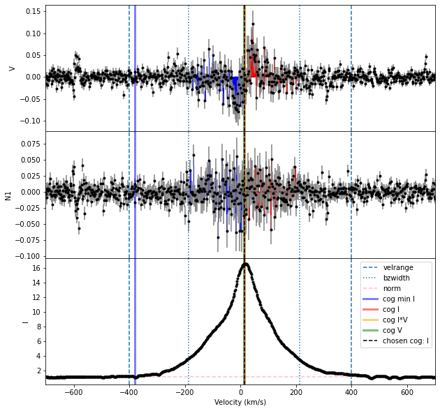
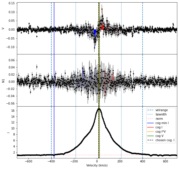
The Halpha line is somewhat complicated to analyze, in that it has a very broad emission component from regions not associated with the magnetic field. This makes the correct velocity range to use for integration in the Bz calculation ambiguous.

For a somewhat cleaner example that is still in a region where two spectral orders overlap, we can look at the He I 587.56 nm line.

# reading the spectrum
spec = pol.read_spectrum("IndividualLine_tutorialfiles/1423137pn.s")
# defining the line parameters
lambda0 = 587.56 ;  geff = 1.0 # He I 587, really a multiplet (so geff is rather approximate)
lwidth = 500. * lambda0 / 2.99e5 #width in nm from width in km/s
# getting the profile for that line
prof = spec.individual_line(lambda0 = lambda0, lwidth = lwidth)

# define the limits for the continuum normalization
# compute Bz in a 50 km/s window around the cog
cogRange = [-100., 150.]
intRange = 50.
Bz = prof.calc_bz(norm = 'auto', cog = 'I', 
                  velrange = cogRange, bzwidth = intRange, 
                  geff = geff, lambda0 = lambda0,
                  plot = False)   

# creating a dataframe to record the result of the different methods in this section
d = {'Merge type':'None'}
d.update(Bz)
df_results = pd.DataFrame(data = [d])

orders = spec.get_orders_in_range(lambda0)
# loop over the individual orders
for ord, type in zip(orders,['lower only', 'higher only']):
    # get the profile for the line in this order
    prof = ord.individual_line(lambda0 = lambda0, lwidth = lwidth)
    Bz = prof.calc_bz(norm = 'auto', cog = 'I', 
                           velrange = cogRange, bzwidth = intRange, 
                           geff = geff, lambda0 = lambda0,
                           plot = False)
    d = {'Merge type':type}
    d.update(Bz)
    df = pd.DataFrame(data = [d])
    df_results = pd.concat([df_results,df], ignore_index=True)

# merging using the trim method
merge = spec.merge_orders(mode = 'trim', midpoint = 0.5)
prof = merge.individual_line(lambda0 = lambda0, lwidth = lwidth)
Bz = prof.calc_bz(norm = 'auto', cog = 'I', 
                  velrange = cogRange, bzwidth = intRange, 
                  geff = geff, lambda0 = lambda0,
                  plot = False)
d = {'Merge type':'trim at mid-point'}
d.update(Bz)
df = pd.DataFrame(data = [d])
df_results = pd.concat([df_results,df], ignore_index=True)

# merging using the coadd method
merge = spec.merge_orders(mode = 'coadd')
prof = merge.individual_line(lambda0 = lambda0, lwidth = lwidth)
Bz, fig = prof.calc_bz(norm = 'auto', cog = 'I', 
                       velrange = cogRange, bzwidth = intRange, 
                       geff = geff, lambda0 = lambda0,
                       plot = True)
d = {'Merge type':'coadd'}
d.update(Bz)
df = pd.DataFrame(data = [d])
df_results = pd.concat([df_results,df], ignore_index=True)

# display the Bz result as a dataframe
df_results.style

using AUTO method for the normalization
  using the median of the continuum outside of the line
using AUTO method for the normalization
  using the median of the continuum outside of the line
using AUTO method for the normalization
  using the median of the continuum outside of the line
using AUTO method for the normalization
  using the median of the continuum outside of the line
using AUTO method for the normalization
  using the median of the continuum outside of the line

/tmp/ipykernel_980312/2408171684.py:13: UserWarning: 
 The velocity array is not monotonically increasing. 
 There might be an order overlap in the region of the observation used. 
 calc_bz will sort the LSD profile in velocity order. 
 Make sure this is what you want -- merge orders before running calc_bz()!
  Bz = prof.calc_bz(norm = 'auto', cog = 'I',

	Merge type	V bz (G)	V bz sig (G)	V FAP	N1 bz (G)	N1 bz sig (G)	N1 FAP	N2 bz (G)	N2 bz sig (G)	N2 FAP	norm_method	norm	cog_method	cog	int. range start	int. range end
0	None	699.503139	66.521645	0.000000	49.584163	66.504701	0.000385	0.000000	0.000000	0.000000	auto	0.991090	I	18.941158	-31.058842	68.941158
1	lower only	822.700767	91.691815	0.000000	-17.652850	91.658895	0.031436	0.000000	0.000000	0.000000	auto	0.992395	I	25.706350	-24.293650	75.706350
2	higher only	793.994679	90.964654	0.000000	220.357069	90.937349	0.002410	0.000000	0.000000	0.000000	auto	0.990170	I	25.578820	-24.421180	75.578820
3	trim at mid-point	797.884180	91.419382	0.000000	221.513065	91.391673	0.002410	0.000000	0.000000	0.000000	auto	0.993520	I	25.587490	-24.412510	75.587490
4	coadd	805.924582	60.001692	0.000000	116.774813	59.981432	0.097482	0.000000	0.000000	0.000000	auto	0.990281	I	25.660364	-24.339636	75.660364