Normalizing a spectrum with normPlot

Before performing an LSD analysis, the observed spectra should be continuum normalized. There are several approaches to this. Here we present the normPlot tool, which can process spectropolarimetric data and has a graphical UI.

About normPlot

normPlot is an interactive graphical tool for normalizing spectroscopic and spectropolarimetric observations, written in Python 3. normPlot can be used as a first step in the SpecpolFlow pipeline, to normalize the continuum of reduced 1D stellar spectra. It is designed to work well with echelle spectra, although it can also work on single-order spectra. normPlot was built to work on one spectral order at a time, essentially establish “good” continuum points, and fit a low order polynomial through those points.

Note

normPlot uses Python 3, version 3.8 or later recommended. Its major dependencies are tkinter and matplotlib. If you installed normPlot with pip, they will likely also be installed, but if they are missing Python will issue an error.

normPlot is an optional add-on for SpecpolFlow, and is not installed by default. You may need to install it with

pip install normPlot

Using the GUI

Note

Prior to using the normalization GUI, the file containing the spectrum should be converted from .fits to .s format (following the LibreESPRIT format). Please see the tutorial on converting to .s files. Tools have been provided for a few commonly used spectropolarimeters.

Command line alternative (if normPlot is not installed with pip)

You can also run the main Python file for normPlot directly, like: python normPlot2.py [observation_file]

Assuming you have installed the program via pip, the interactive normalization UI can be started from the terminal with the command

normplot [observation_file]

You can also run normPlot from within a Jupyter Notebook or other Python script

import normPlot
normPlot.normplot('[observation_file]')

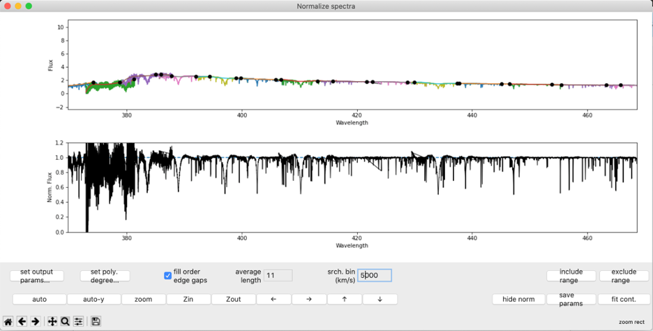
Once executed, you should see the following window appear

The top panel of this window displays the observed spectral orders (in different colors), the black points used for actual fitting, and polynomial fits for each order. The black fitting points are computed by dividing an order into consecutive search bins of equal width and extracting the maximum flux within each bin. The panel below is a preview of the normalized spectrum that would be output by the code. The axes are synced and allow the user to compare the unnormalized and normalized spectrum in the same range of wavelengths. The lower panel updates anytime the new fit is explicitly computed. Wavelengths are in the units of the input observation (in this case nanometers).

Buttons in the interactive UI

There are controls for navigating the GUI plot: auto (automatically scales the axes), auto-y (scales the y-axis only), Zin (zoom in), Zout (zoom out), and panning buttons (left, right, up, and down). These also have keyboard shortcuts (e.g. arrow keys pan), see the tooltips for the buttons. The matplotlib default toolbar below these buttons also works for navigating the frame home position, revert step, redo step, pan, zoom, and snapshot.

There are several buttons for interactively improving the polynomial fits and normalization.

Fit cont.

Clicking this button will apply any parameter changes made and update the continuum fit. This will simultaneously update the final normalized spectrum.

set output params

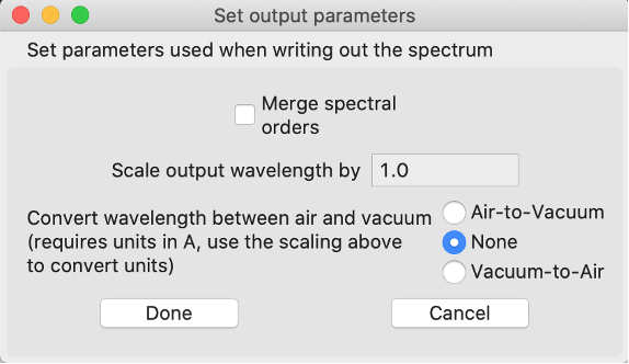
Here you can determine the structure of the spectrum in the output file. If you select Merge spectral orders the final spectrum will be continuous rather than separate orders (if separate, there will be wavelength overlap between consecutive orders). In the process of merging the orders, where there is overlap, the program uses the first order up to the middle of the overlap then uses the second. The lower plot in the main window will change accordingly, so you will be able to preview the merged normalized spectrum. The wavelength units can also be scaled (e.g. to convert from nm to A set the scale to 10). The wavelengths can also be converted between air and vacuum wavelengths, however this requires wavelengths in angstroms (if you have wavelengths in nm: set the scale wavelengths value to 10, then it will apply scale before the air-vacuum conversion).

set poly. degree

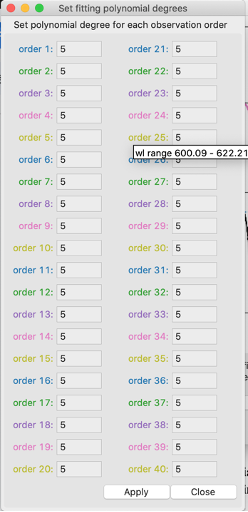
Here the degree of the individual polynomials can be set for each order. The color of the text corresponds to the color by which that order is plotted. If you hover your mouse over one of the inserts, text will pop up indicating the wavelength range for that given order. This will help in searching for a specific order on the plot. After clicking apply, and then fit cont., you will see a change in the polynomial plotted over the order (and in the normalized spectrum in the region corresponding to that order).

fill edge order gaps

This check box enables a feature for dealing with spectral orders that end in an exclude region. The algorithm can take a fitting point in the adjacent spectral order and use that to constrain the continuum polynomial. This can be useful around very broad features like Balmer lines.

srch. bin (km s\(^{-1}\))

This value sets the width of the search bins, in velocity units. The code selects only one point in each bin for actual fitting. It takes the point with the highest flux as (hopefully) being most likely real continuum. As you increase the width of the bins, you decrease the number of fit points for each order and vice versa. The search bin should be set large enough that there is generally some real continuum in the bin.

average length

Within all the search bins, the code applies boxcar averaging to smooth the data before extracting the best point to fit (max. flux). This input sets the width (i.e. number of neighboring data points in the spectrum) that will be used in the averaging. This is useful for correcting selected fitting points that favor noise, and fall a bit too high. This smoothening is only used when computing points to fit polynomials through, so you will not produce a smoothed normalized spectrum.

exclude range

You can select specific ranges of wavelength to be excluded from the fitting process. After clicking this option and going into either panel, the first click will set the starting edge of the exclusion range. A box made of dashed lines will appear with one edge fixed on where the first click. The second vertical edge will follow the mouse in the panel, and all wavelengths within this box will be excluded. A second click will finalize this selection and after pressing fit cont. you will see that enclosed portion of the spectrum change its color to black (this signifies that it is not included in the fitting). Any fit points in that enclosed region will also disappear. If you are partway through selecting a region (clicked once but not twice), you can right click to cancel the selection.

include range

This provides a way to reverse the exclusion function. You can selected ranges within excluded regions to be un-excluded when the normalization is updated.

hide norm

You have the option to remove the lower panel (or return it) at your leisure. The upper panel will expand to the height of the full window. This feature can be useful for doing normalization with a small computer screen.

save params

The chosen parameters (after fitting) can be saved to the files: exclude.dat, poly-deg.dat, and params.dat. These files can later be loaded to start from where you left off, or for a good initial guess if you are normalizing similar spectra. Usually it’s safest to always click this button before closing the main window, just in case you want to tweak a normalization later. (Closing the main window always automatically saves the normalized spectrum.)

Output files

Once the main window is closed the program will save the normalized spectrum to [observation_file].norm.

Note

The output will use the normalization and parameters of the last update. It is advised that you use the fit cont. button before closing the window.

If you clicked the save params, the program will also write out the fitting information in the files, mentioned above. It’s is useful to make a copy of these files with a name unique to the data.

Running normPlot with previous parameters

When running normPlot again, it will check for the prameter files and try to read them if they exist: exclude.dat, poly-deg.dat, and params.dat. Alternatively, you can run normPlot using copies of those files with specified names from the command line:

normplot -e [exclude_file] -d [poly-deg_file] -c [params_file] [observation_file]

or within Python:

import normPlot
normPlot.normplot('[observation_file]',
                  excludeRegionName='[exclude_file]', 
                  polynomialsName='[poly-deg_file]', 
                  paramsName='[params_file]')

You can also take the parameter files and apply them to spectra without having the reopen the interface. This uses the -b flag from the command line:

normplot -b -e [exclude_file] -d [poly-deg_file] -c [params_file] [observation_file]

or the batchMode=True argument in Python:

normPlot.normplot('[observation_file]',
                  excludeRegionName='[exclude_file]', 
                  polynomialsName='[poly-deg_file]', 
                  paramsName='[params_file]',
                  batchMode=True)

This useful for normalizing a large number of observations of the same object.