From normalized spectrum to Bz measurement

From normalized spectrum to Bz measurement#

In the below code, we will walk through how to use SpecpolFlow (with the use of LSDpy) with a single, normalized Stokes V spectrum for the magnetic B star \(\xi^1\) CMa (HD 46328; Erba et al. 2021; ESPaDOnS). The code has the following structure:

Import packages
Star Selection
Creating the LSD Line Mask
Cleaning Line Mask
Creating LSD Profile
Extracting \(B_{\text{z}}\)

First, we need to import the packages:

1. Necessary information and files#

To use this tutorial, you must start with a normalized spectrum in the so-called ‘Donati’ format (a ‘.s’ file). If you do not have a ‘.s’ file (you have ‘.fits’ or ‘.p’ files), please see the previous tutorial: Normalizing a spectrum with normPlot.

Collect ‘.s’ file. For this example, we provide the file (hd46328_test_1.s). For our example, the stellar parameters of are:
- \(T_{\text{eff}}\) = 27000 K
- \(\log g\) = 3.5 (cgs)
- \(v\sin i\) = 15 km \(\text{s}^{-1}\)
- \(\text{RV}\) = 12 km \(\text{s}^{-1}\)
Collect important stellar parameters:
- \(T_{\text{eff}}\), log g are necessary to obtain the line list for the LSD mask
- You might also find it useful to have the \(v\sin i\) and observation specific radial velocities (however these can be measured later on the the LSD profile).
Next we will need to obtain a list of atomic and molecular transition parameters for this \(T_{\text{eff}}\), log g from the Vienna Atomic Line Database (VALD; Ryabchikova et al. 2015). The line list for this star is provided (LongList_T27000G35.dat),

Need to download your own line list?

To retrieve a VALD line list, click the “Extract Stellar” button on the VALD website.

Note

You need to register an email to access the site.

In our example, we use the following input to obtain the line list:

Starting wavelength: 3700 Å
Ending wavelength: 9000 Å
Detection threshold: 0.01 (line depths shallower than this threshold are not included)
Microturbulence: 2 km s\(^{-1}\)
\(T_{\text{eff}}\) = 27000 K
\(\log g\) = 3.5 (cgs)
Chemical Composition: 0.0 [Fe/H] (Solar)
Long format
Linelist configuration: Default

The long format line list file is a text file consisting of a header line containing information on the wavelength range of the list, as well as other information about the content of the file.

For each spectral line, there is a row of information about the physical parameters like the energy levels involved, the measured Landé factors, etc. Then two rows with information about the electron configurations and term symbols, and a row with references.

To create LSD profile, we need some specific information about each spectral lines, and the tools described in the next section will transform the VALD files into a Mask file.

2. Creating LSD Line Mask#

To convert the VALD long format line list file into a LSD line mask file, we use the make_mask function. We need to specify the location and name of the input VALD file and the output file.

We will use the options depthCutoff (which only selects lines with depths greater than the specified value), and atomsOnly (atomsOnly = True excludes H lines and molecular lines). For additional options, please consult the make_mask API.

This will create a mask file (we suggest to give the output file a .mask extension).

VALD_file_name = 'OneObservationFlow_tutorialfiles/LongList_T27000G35.dat'
file_output = 'OneObservationFlow_tutorialfiles/test_output/T27000G35_depth0.02.mask'
mask = pol.make_mask(VALD_file_name, outMaskName = file_output, depthCutoff = 0.02, atomsOnly = True)

missing Lande factors for 160 lines (skipped) from:
['He 2', 'O 2']
skipped all lines for species:
['H 1']

3. Cleaning the Line Mask#

Next, we remove sections in the mask that we do not want affecting the LSD profile. For example, these include:

regions 400 km s\(^{-1}\) (specific to this example) around the Balmer series
the Balmer jump where the spectrum normalization is not great
areas of large telluric contamination.

We remove these sections because the lines are either of the wrong shape or the data is contaminated by the earth’s atmosphere; both would negatively effect later processing.

In this example, we will use default regions that are available in SpecpolFlow:

We can exclude the Balmer using the get_Balmer_regions_default function. This function takes in the velocity region around the line center that you want to exclude. In our example, we will use 400 km/s on each side of the line, to exclude any other spectral lines that would be in the broad wings of the Balmer lines.
We can exclude the telluric regions with the get_telluric_regions_default.

Then the Mask.clean class function removes the lines within regions specified. The clean mask can now be output to a new .mask file using the Mask.save class functionality.

# get some regions to exclude from the mask
velrange = 400.0 # units are in km/s
# get both the Balmer and telluric regions, and combine them 
excluded_regions = pol.get_Balmer_regions_default(velrange) + pol.get_telluric_regions_default()

# visualization of excluded regions
pd.DataFrame(excluded_regions.to_dict())

	start	stop	type
0	655.405353	657.156647	Halpha
1	485.491365	486.788635	Hbeta
2	433.470866	434.629134	Hgamma
3	409.622728	410.717272	Hdelta
4	396.480287	397.539713	Hepsilon
5	360.000000	392.000000	Hjump
6	587.500000	592.000000	telluric
7	627.500000	632.500000	telluric
8	684.000000	705.300000	telluric
9	717.000000	735.000000	telluric
10	757.000000	771.000000	telluric
11	790.000000	795.000000	telluric
12	809.000000	990.000000	telluric

# location of the output file
clean_Mask_filename = 'OneObservationFlow_tutorialfiles/test_output/hd46328_test_depth0.02_clean.mask'

# run cleanMask function
mask_cleaned = mask.clean(excluded_regions)
# and save the cleaned mask
mask_cleaned.save(clean_Mask_filename)

Tip

For more information about the functionalities of the Mask and ExcludeMaskRegion class objects, see the tutorials:

Tip

For a more careful detailed approach to cleaning a mask, you can use the interactive tool cleanMaskUI, see

How to clean masks with the interactive tool

If you are doing a detailed analysis of a star, we recommend using this!

4. Creating the LSD Profile#

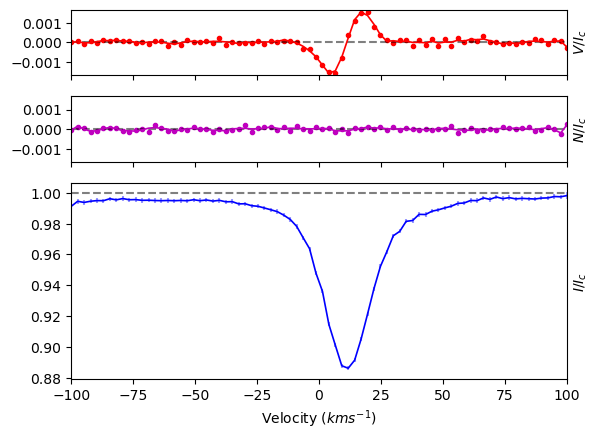
Least-Squares Deconvolution (LSD) is a cross-correlation technique for computing a profile similar to the weighted average of selected spectral lines (Donati et al. 1997).

To compute an LSD profile, we need to define the normalizing weights that will be used. In this example, We use these commonly used values:

normDepth = 0.2 — normalized line depth
normLande = 1.2 — normalized effective Lande factor
normWave = 500.0 — normalized wavelength

To capture the entire line profile, we set the range of the LSD profile to 100 km s\(^{-1}\), because we know that the \(v\sin i\) star is 15 km s\(^{-1}\).

Additionally, the pixel size should be set relative to the resolution and pixel size of the data; for ESPaDOnS data, we should not go below the 1.8 km s\(^{-1}\) pixel size. In a case where the line profile is very broad, it may be advantageous to use larger pixels, it is important to make sure the profile is sampled with enough datapoints. For our example, we use 2.6 km s\(^{-1}\) per pixel.

To calculate the LSD profile, we call the run_lsdpy function.

Warning

The run_lsdpy function only works using the mask (‘.mask’) and spectrum (‘.s’) files as input: you cannot pass an already loaded Spectrum or Mask objects as input.

The run_lsdpy function returns an LSD object, as well as the model spectrum as a Spectrum object.

In the below code, we also specified the name and location for saving the LSD profile into a file (‘.lsd’).

We leave all of the other parameters to their default values. For full description of LSDpy options, see LSDpy.

clean_Mask_filename = 'OneObservationFlow_tutorialfiles/test_output/hd46328_test_depth0.02_clean.mask'
spectrum = 'OneObservationFlow_tutorialfiles/hd46328_test_1.s'

LSD_outfile = 'OneObservationFlow_tutorialfiles/test_output/hd46328_test_1.lsd'

lsd, mod = pol.run_lsdpy(obs = spectrum, mask = clean_Mask_filename, outLSDName = LSD_outfile, 
           velStart = -100.0, velEnd = 100.0, velPixel = 2.6, 
           normDepth = 0.2, normLande = 1.2, normWave = 500.0)

Tip

If you are, e.g., making tests and do not need to save the resulting LSD profiles to files just yet, simply keep the returned LSD profile and Model Spectrum as variables and don’t set the outLSDName and outModelNamekeywords. You can save later on with the LSD class save function.

lsd, mod = pol.run_lsdpy(obsFile, maskFile, ...)

[more manipulation of the lsd object]

lsd.save('Name of file')

If you are, e.g., only interested in generating LSD files and do not need to do further manipulations in the code, then you do not have to store the returned LSD object and Model Spectrum object as variable.

pol.run_lsdpy(obsFile, maskFile, outLSDName = 'Name of File', outModelName = 'Name of file')

5. Calculate \(B_z\) from LSD Profile#

To calculate the longitudinal field \(B_z\) from our LSD profile, we will use the calc_bz function of the LSD class.

To compute \(B_z\), we need to know the velocity (or center-of-gravity ‘cog’) of the center of the spectral line, and the characteristics of the line (normalizing wavelength and Landé factor \(\lambda_0\), \(g_\text{eff}\)). It is also customary to renormalize the LSD profile to the continuum surrounding the line.

In our example here, we will use the default built-in methods to compute the cog (cog = 'I') and the continuum normalization (norm = 'auto').

Note

For other options, see How to calculate the longitudinal field and False Alarm Probability and the calc_bz API.

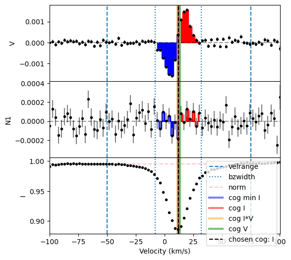
To use the automated methods, we will give calc_bz the velrange keyword. This defines the range of velocity to use for the determination of the cog with built-in method, and the range to exclude in the built-in normalization. In our case here, we will use the default method cog = I, and as the spectral line is roughly between -50 km s\(^{-1}\) to 75 km s\(^{-1}\), so we will use velrange = [-50.0, 75.0].

The calculation of the longitudinal field and FAP uses the bzwidth keyword, which should be set to include just the line itself. This keyword sets a velocity range from the cog value (equal distance if it is set to a single number, distance to the blue and red side of the line is set to a 2-item array). That range from the cog is used to integrate the Bz equation, and evaluate the FAP. In our case here, we will set the range of the integration to be 20 km/s on each side of line center, therefore we set bzwidth = 20.0.

Finally, we set plot = True to output a diagnostic plot.

LSD_outfile = 'OneObservationFlow_tutorialfiles/test_output/hd46328_test_1.lsd'

# Bz calculation using manual cog selection
velrange = [-50.0, 75.0] # the velocity range over which the center line is found
bzwidth = 20.0 # this is the width about the center line used to calculate Bz

lsd = pol.read_lsd(LSD_outfile)
Bz, fig = lsd.calc_bz(cog = 'I', norm ='auto', velrange = velrange, 
                      bzwidth = bzwidth, lambda0 = 500.0, geff = 1.2,
                      plot = True, figsize = (6,6))

using AUTO method for the normalization
  using the median of the continuum outside of the line

The function outputs a dictionary with the following content:

V bz: Bz (G) calculated from Stokes V profile
V bz sig: (G) standard deviation
V FAP: false alarm probability FAP (Donati et al. 1997). Definite detection (DD) is defined as having a FAP \(< 10^{-5}\). A non-detection (ND) is defined as having a FAP \(> 10^{-3}\). FAPs between \(10^{-5}\) and \(10^{-3}\) are defined as a marginal detection (MD).
Null calculations - N1 and N2 are two different methods for null profile calculations; N1 is most commonly used.
- N1 bz: Bz (G) calculated from the Null 1 profile
- N1 bz sig: (G) standard deviation
- N1 FAP: false alarm probability of Null 1
- N2 bz: Bz (G) calculated from the Null 2 profile
- N2 bz sig: Bz (G) standard deviation
- N2 FAP: false alarm probability of Null 2
norm_method: a record of the method used for the normalization
norm: continuum value used for normalization
cog_method: a record of the method used for the determination of the cog
cog: the center of gravity value
int. range start (km s\(^{-1}\)): lower bound of the velocity range used for the Bz and FAP calculation
int. range end (km s\(^{-1}\)): upper bound of the velocity range used for the Bz and FAP calculation

We can convert the returned dictionary into a Pandas dataframe for an easy display

pd.DataFrame(data = [Bz]).style

	V bz (G)	V bz sig (G)	V FAP	N1 bz (G)	N1 bz sig (G)	N1 FAP	N2 bz (G)	N2 bz sig (G)	N2 FAP	norm_method	norm	cog_method	cog	int. range start	int. range end
0	-111.841454	4.119598	0.000000	-3.723758	4.041478	0.274214	0.000000	0.000000	0.000000	auto	0.995431	I	11.945350	-8.054650	31.945350

To see additional capabilities of the Bz function, see How to calculate the longitudinal field and False Alarm Probability and the calc_bz API.