How to clean masks with the interactive tool#
Introduction#
This tutorial will introduce you to the interactive mask cleaning tool called cleanMaskUI. This tool allows regions of lines to be easily excluded and included in the LSD line mask. This is particularly useful in the case of stars with a lot of emission: since emission lines have a different shape than the typical absorption lines, they should not be included in the line averaging since they will distort the resulting LSD profile. For this tutorial we will use the star HD 164284, a Classical Be star with a spectrum that is contaminated by emission lines from a disk.
cleanMaskUI can be run from either from the command line, or from a Python file, or a Jupyter Notebook.
The cleanMaskUI function takes:
The file name of your line mask, or the corresponding Mask object
The file name of an observed spectrum ‘.s’ file, for comparison and LSD calculations
The file name for saving the new cleaned mask (optional; if not specified it will use the input mask name with ‘.clean’ added)
The exclude mask region file, which contains the set of regions to be excluded from the mask (optional)
For running the tool from the terminal use:
spf-cleanmask input_mask_file reference_observation.s cleaned_mask_file
For running the tool from inside a Python or Jupyter Notebook use:
import specpolFlow as pol
pol.cleanMaskUI('input_mask_file', 'reference_observation.s', 'cleaned_mask_file')
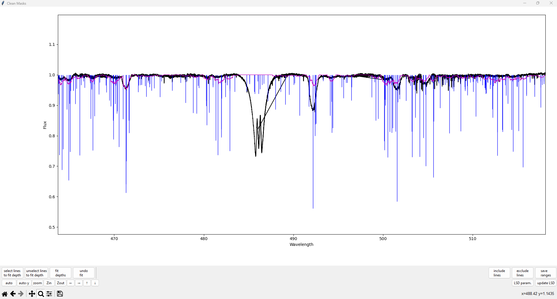
Running the code opens a new window, with a GUI that will look like this:
The vertical lines indicate the locations and depths of spectral lines in the input line mask. Lines colored blue indicate that they are being used (with iuse=1), and lines colored red indicate that they are not being used (with iuse=0). The black line is the observed spectrum, and the purple line is the model LSD spectrum (i.e. the spectrum created by convolving the LSD profile with the line mask).
Including and Excluding Lines#
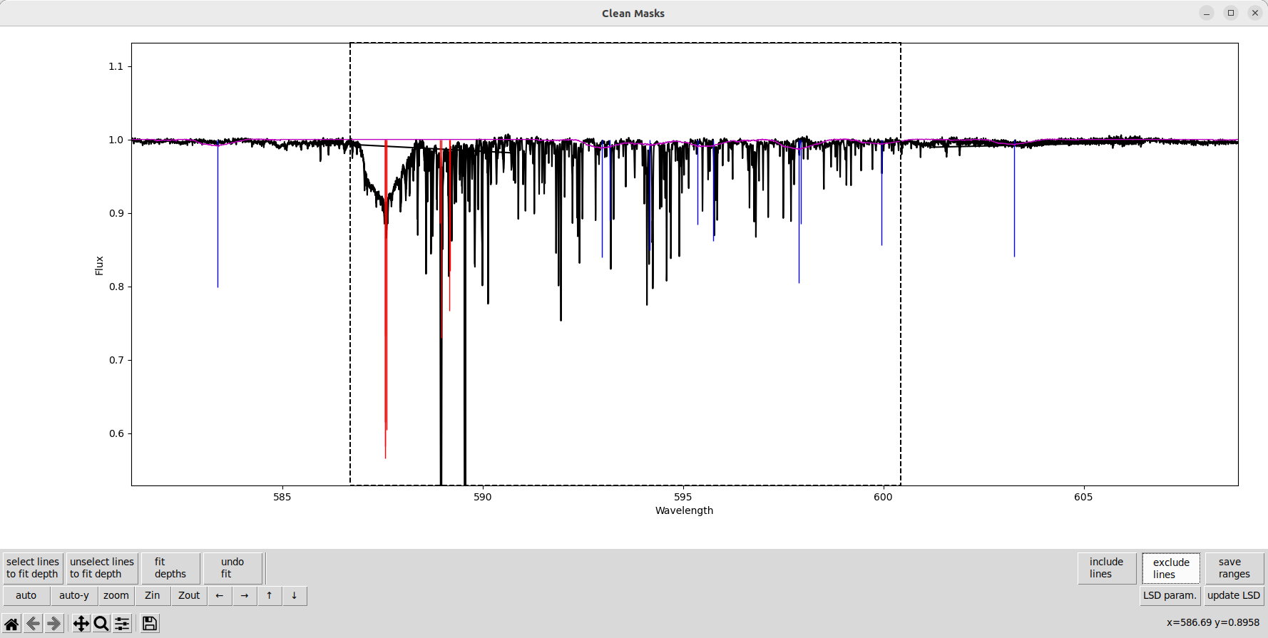
Lets now manually exclude a region around that emission line. On the bottom right, click the exclude lines button. The button should now have a dotted box around it indicating that it is active, as shown below.

Click on the plot to create a vertical dotted line indicating one edge of the region. Then, click on another part of the plot to finish selecting the region. The region selection is shown below.
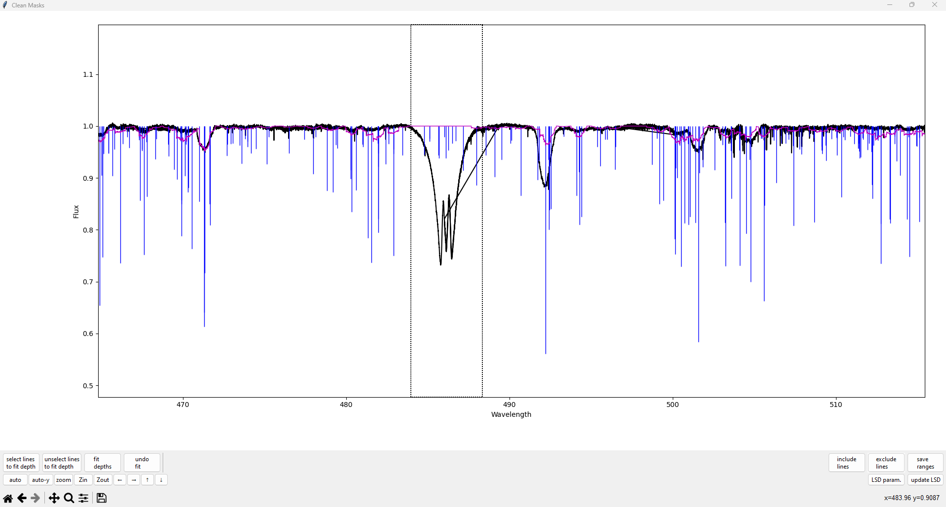
After the second click to close the region, all spectral lines within the selected region should now turn red. (You can also right click during the selection, after the first click, to cancel.)
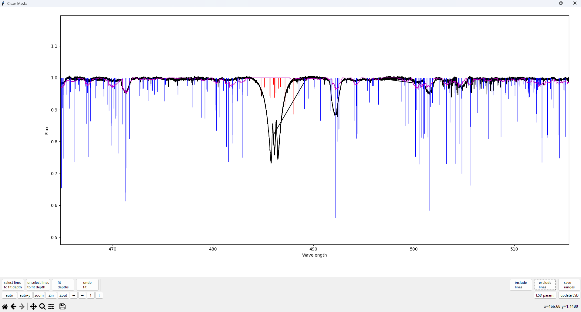
Once you have finished selecting regions to exclude, don’t forget to click the exclude lines button again to deselect that mode. You should see the dotted box around the button (and lighter color) disappear. Note that the custom buttons for panning and zooming will work while the ‘exclude lines’ mode is active, but the default matplotlib toolbar at the very bottom does not.
The above procedure works exactly the same for the include lines button. That button will add lines back into the mask, in other words it will turn the red (excluded) lines back to blue (included).
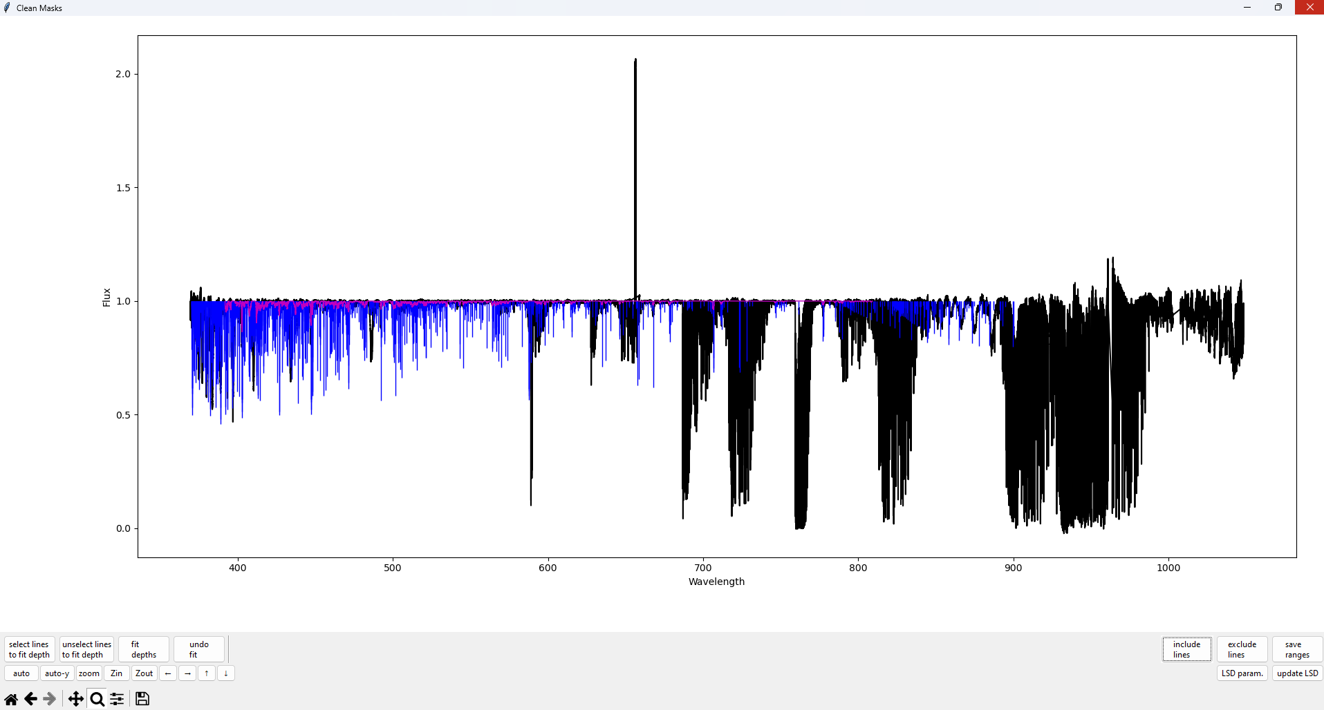
By default, lines in some commonly problematic regions (around telluric lines and Balamer lines) are excluded. In some cases it may be helpful to include those lines. In other cases you may want exclude additional wider regions.
Updating and Plotting the LSD Profile#
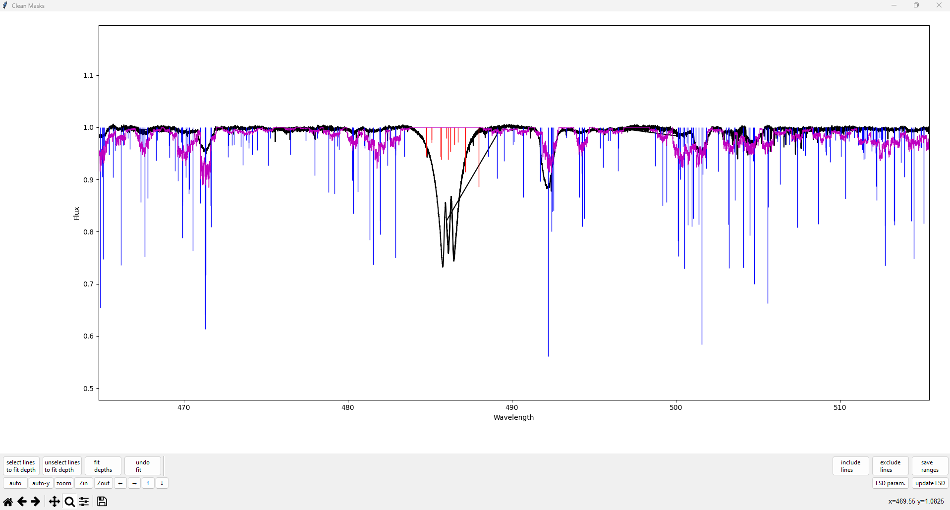
Once we have selected the regions to exclude, we can update the test LSD profile by clicking the update LSD button in the bottom right. This will update the purple model spectrum line as shown below and update the output cleaned mask.
We can also adjust the input parameters for the test LSD profile by selecting the LSD param button in the bottom right. This will open another window titled Set LSD parameters as shown.
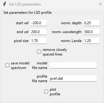
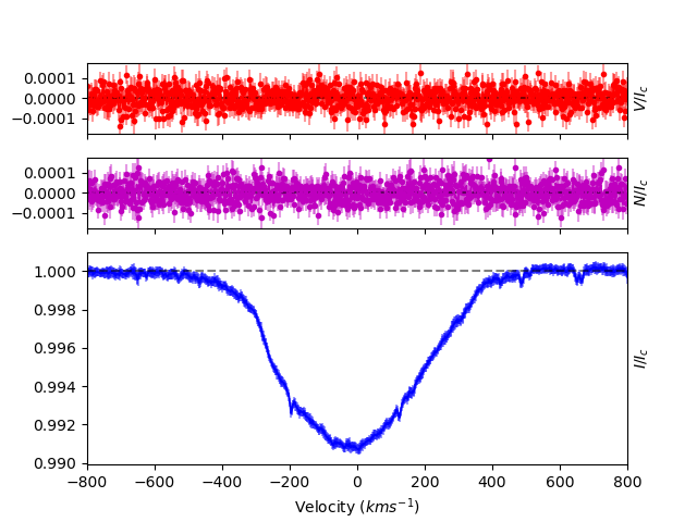
In this example we will change the starting and stopping velocity to \(\pm\) 800 km s\(^{-1}\), since this Be star has an extremely high \(v\sin i\). We also select the remove closely spaced lines and plot profile boxes. The latter box will plot the test LSD profile every time the update LSD button is pressed. In a Jupyter Notebook this LSD plot should be visible back in the cell output where the cleanMaskUI function was executed.
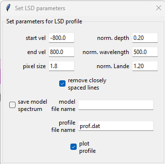
Close the Set LSD parameters popup window and select update LSD to update the model spectrum and create an LSD plot.
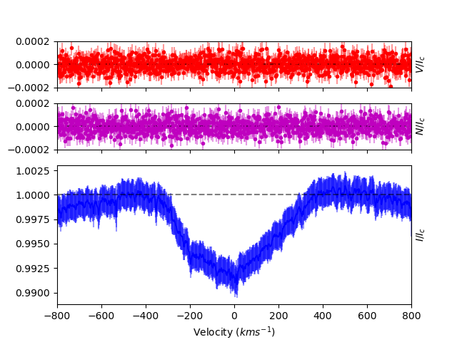
Since only one emission line was removed, and since no other lines were changed, the LSD profile is still distorted, and noisy with large errorbars. However, after doing a thorough pass through the whole spectrum, a useful LSD profile can be obtained.
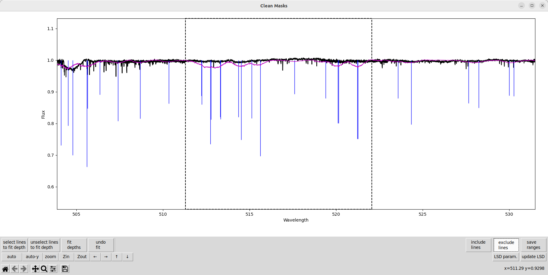
Since the lines are relatively shallow in this star, we remove more lines blended with weaker telluric lines.
We also remove some lines where the line depths are wrong and the lines aren’t clearly seen in the observation. In this star, that is partly due to the very high \(v\sin i\).
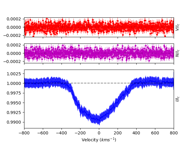
After going through the entire spectrum, removing more problem regions, we get a much better LSD profile.
Automatically Adjusting Line Depths#
Sometimes it can be helpful to use empirical estimates of line depths for some lines in the mask. The theoretical line depths could be wrong due to NLTE effects, errors in the atomic line data, or desaturation/broadening effects that weren’t accounted for.
In cases where many lines in the mask have depth problems, it is usually better to improve the theoretical depths going into the mask. It is important to have the correct effective temperature and \(\log g\) for the mask. If the star has chemical peculiarities it is important to account for those too. This can be done within a VALD extract stellar request. You may also wish to consider more elaborate spectrum synthesis calculations for the line depths, particularly if NLTE effects are very important.
In general empirical line depth estimates should be used with caution. There is a good reason for your choice of theoretical line depths (or there should be!). Furthermore, there is an intrinsic degeneracy between the depths of the lines in the mask and the amplitude of the LSD profile. In cleanMaskUI this is resolved by simply assuming the current LSD profile is an adequate approximation when fitting line depths. This means that if your initial LSD profile (from the initial line mask) is too poor quality, then depth fitting will produce poor results. This also means that one should only fit carefully selected problem lines, not all the lines in the mask.
In our example Be star, fitting depths of some lines can be quite helpful. Since \(v\sin i\) is quite large there are relatively few clearly detected lines in the spectrum, so depth errors in some of those lines can have a large impact.
To automatically fit line depths, click the select lines to fit depth button, then click on the plot to begin selecting a range of lines, then click on the plot a second time to finish selecting lines. The selected lines in the mask should turn light blue. Then click the fit depths to fit the depths of all selected lines (light blue) simultaneously.

Here is a line that is clearly present in the observation but has a depth that is too weak. We select the line, and a few neighboring blended lines.
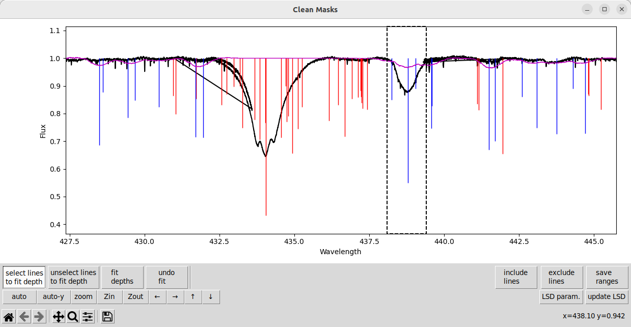
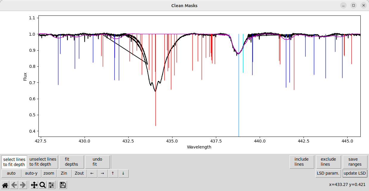
Then, after selecting the line we click fit depths, then click update LSD to see how these new depths match the observation. The updated fit to the observation is pretty good.
Note
The select lines to fit depth button remains active until you click it a second time to deactivate the mode (or click the unselect lines to fit depth to switch modes). This is similar to the exclude lines and include lines buttons.
There are some lines that are too strong in the model, and very weak (but still present) in the observation. Here we select a set of those problem lines.
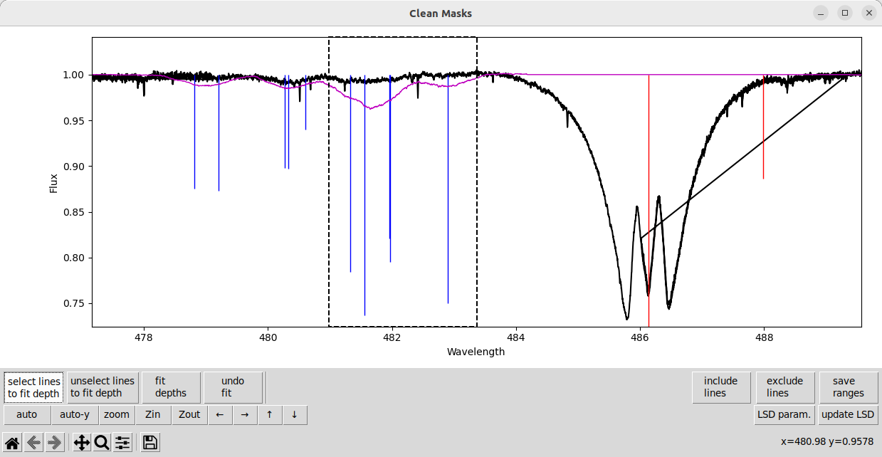
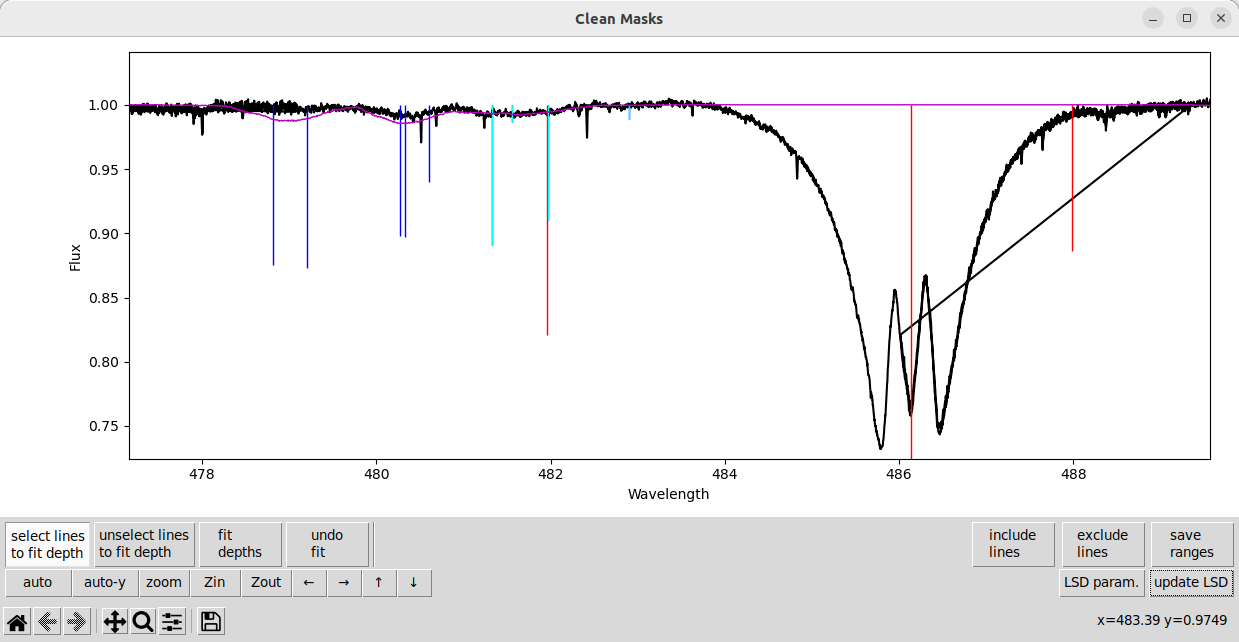
And then fit the depths for them, and update the LSD calculation.
The line depth fitting routine can struggle with heavily blended lines. Fitting blended lines is usually not a fully degenerate problem, but it can ambiguous how much of the depth to assign to which line. This can cause the wrong line to be made strong or weak, and it can even cause depths to become negative!
Note
Fitting depths for lines with virtually the same wavelength can be fully degenerate. In this case, the fitting routine will automatically exclude the weaker line from the mask so that fitting can proceed.
Here is a strong line where we would like to fit the line depth(s) but it is blended with several other lines.
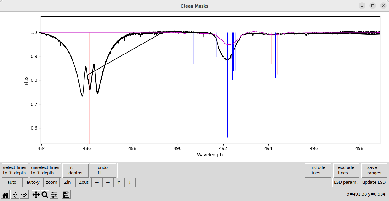
We can select the lines in the mask and fit them. But some of the line depths becomes negative! The negative line depth is indicated by the light blue line in the plot that goes up from 1, rather than down. This may be numerically the best fit, but clearly this is a non-physical solution.
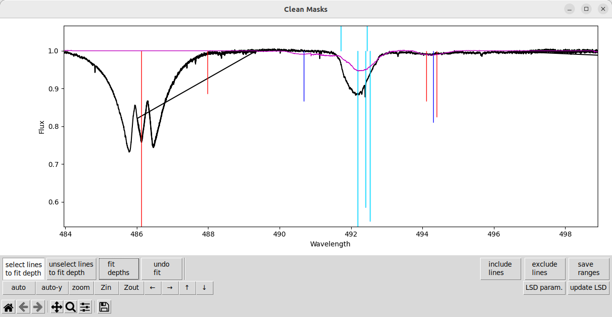
First we need to undo the fit, by pressing the undo fit button. Then we want to remove some lines from the fit using the unselect lines to fit depth button. The lines should turn a darker blue when unselected.
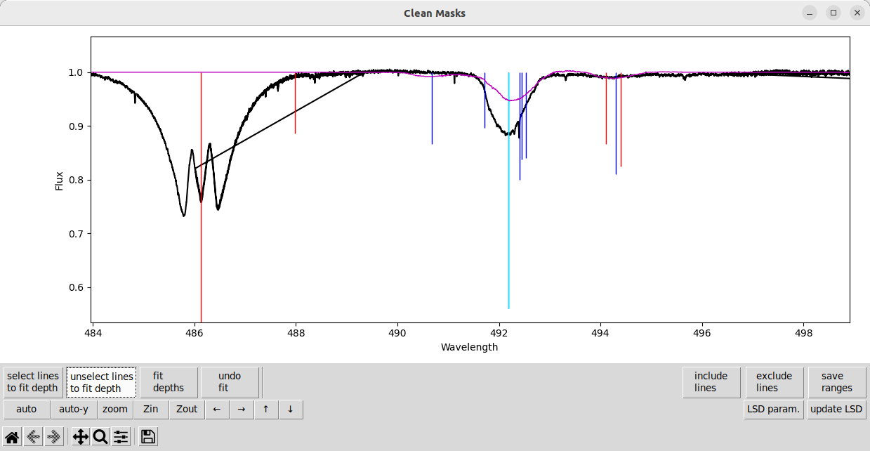
If we just fit the depth of the one strongest line, and then update the LSD calculation, we get something pretty close to the observation.
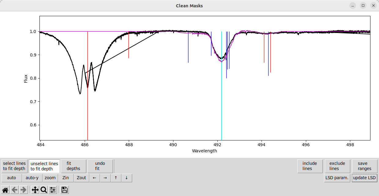
Although the model is a little too deep for the observation now. That is because the lines not selected for fitting are completely ignored when fitting line depths. So the weak lines’ contribution to the blend is is not accounted for when fitting the stronger line.
In this case, the line is dominated by the strong component, so we can simply exclude the weak components from the mask. This slightly improves the fit to the observation.
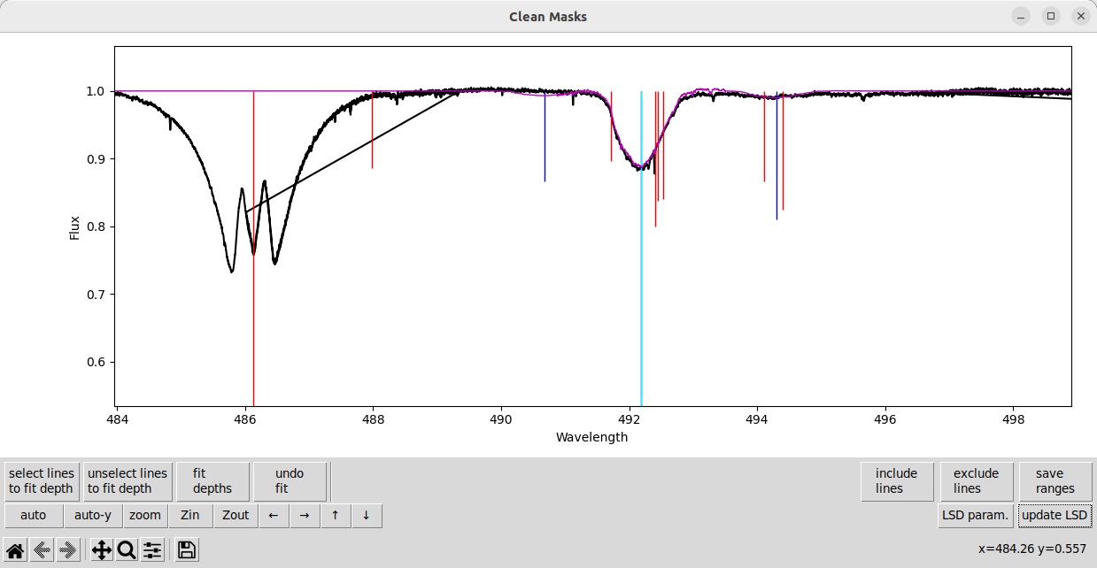
In other complex cases, it may be optimal to fit the depths of multiple stronger components of a blend, but exclude weaker components from the mask.
After tweaking the depths of several more lines across the spectrum, we get an improved LSD profile. Because the better depths improve the fit to the observed Stokes I spectrum, the errorbars for the Stokes I LSD profile are much smaller. Also, because a lot of the signal in the observation was in a few He lines with poor depths, the S/N in Stokes V is noticeably better.
When you are done, closing the window automatically saves modified mask with the final fit depths. The output mask is saved using either the output name you provide, or using original mask name with ‘.clean’ added to the end.
