Calculating line bisector from LSD profiles and individual lines

Line bisectors can be useful to study line asymmetries induced by photospheric convection. For example convective blueshift, caused by the imbalance in surface coverage between hot granules (rising material) and cooler intergranular lanes (downflow material). In this tutorial, we explore how the bisector function calc_bis, part of the LSD class, can be used to analyse LSD profiles as well as individual lines.

First import specpolFlow and any other packages.

Show code cell content Hide code cell content

import specpolFlow as pol

import matplotlib.pyplot as plt
import numpy as np

Computing bisectors on LSD profiles

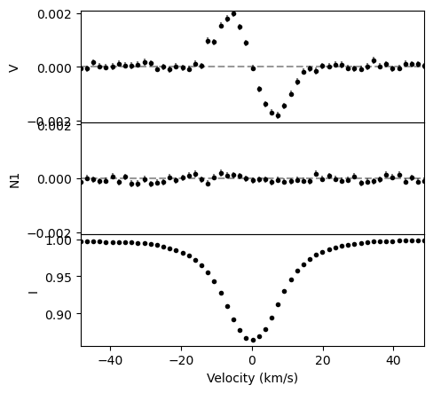
For our first example, we provide an LSD profile (SampleLSD.lsd) to illustrate the use of bisectors. First, we load the LSD profile, shift it to the stellar reference frame, and adjust the continuum normalization.

# read the LSD profile
lsd = pol.read_lsd("CalculateBz_tutorialfiles/SampleLSD.lsd")
# estimate the systemic velocity using the center of gravity of Stokes I
cog, cog_err = lsd.cog_rv([15.0, 95.0])
# Doppler shift the profile 
lsd = lsd.vshift(cog)
# continuum normalization
lsd = lsd.norm(np.median(lsd.specI[(lsd.vel < -50.0) | (lsd.vel > 50.0)]))
# slice profile to select a smaller window
lsd = lsd[np.abs(lsd.vel) < 50.0]
fig, ax = lsd.plot(figsize = (5,5))

We use the calc_bis function to compute the line bisector and velocity span following the definition of Gray (1982) and Queloz et al. (2001), respectively. The biswidth keyword specifies the velocity range around the cog (i.e. relative to the line center) that will then be used to compute the bisector. Other possible kwargs are plotFit and fullOutput.

Note

The velocity span is the difference from the average velocity at the top and bottom part of the line bisector; this can be viewed as an estimation of the inverse of the mean slope of the bisector.

By default, fullOutput = False and only the velocity span and its uncertainty are returned. One can also set fullOutput = True to return:

• velocity span and its uncertainty

• top velocity (i.e., within 10–40 per cent of the full line depth)

• bottom velocity (i.e., within 60–90 per cent of the full line depth)

• line bisector array

• intensity levels at which bisectors were computed

# compute the line bisector in a 40 km/s window around cog
biswidth = 40.0

# get the velocity span and plot the line bisector
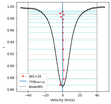
vspan, vspan_std = lsd.calc_bis(cog=0.0, Ic=1.0, biswidth=biswidth, fullOutput=False, plotFit=True)

print("Velocity span = {:1.3f} +/- {:1.3f} km/s".format(vspan, vspan_std))

# get the full set of optional outputs
vspan, vspan_std, vtop, vbottom, vel_bis, int_bis = lsd.calc_bis(cog=0.0, Ic=1.0, biswidth=biswidth, fullOutput=True)

Velocity span = -0.054 +/- 0.050 km/s

The figure above shows a few useful things:

• vertical blue line shows the cog used as the line center

• black dotted line shows the velocity width used to compute the bisector

• horizontal cyan lines in the figure represent the intensity levels used to compute the line bisector - Note that the line profile must be interpolated at the left and right intersections with these levels to compute the bisector

• red line illustrates the line bisector, scaled up by a factor for illustration purposes.

Warning

It is important to adequately set the continuum level Ic as the bisector function uses that value as a reference to estimate the velocity span.

Computing bisectors for individual line profiles

The following example demonstrates how to use bisectors on individual spectral lines. We analyze the spectrum of the main-sequence G-type star 51 Peg, the first star where an exoplanet was detected. Although not covered in this tutorial, bisectors are a valuable tool for determining if radial velocity variations are due to an orbiting planet. The planet reflex motion should only shift the line bisector without modifying its curvature or velocity span. So correlations between the velocity span and the radial velocity help identify cases where signal from a planet candidate is really from stellar activity.

# read the spectrum
spec = pol.read_spectrum("CalculateBisector_tutorialfiles/1604052pu.s.norm")

First create individual line profiles for a couple of iron, sodium and hydrogen lines. We use the individual_line function of the Spectrum object to do this, which is described in more detail in How analyze individual spectral lines.

# define the line parameters
line_ref = ['Fe I', 'Fe I', 'Na I', 'Fe I', 'Fe I', 'Fe I', 'Fe I', 'Fe I', 'Halpha']
lambda0 = [539.318, 543.4523, 589.5924, 617.333, 602.70505, 624.633, 625.256, 630.2493, 656.281]

# radial velocity (center of gravity) from literature
cog = -33.129

# compute the line bisector in a biswidth window around cog (km/s)
biswidth = [20.0, 20.0, 30.0, 15.0, 15.0, 15.0, 15.0, 10.0, 40.0]

profs = []
# loop over each line, and each biswidth value
for il0, ibiswidth in zip(lambda0, biswidth):
    lwidth = 150.*il0/2.99e5 #get a 150 km/s width around the line, in nm

    # get the profile for this line
    iprof = spec.individual_line(il0, lwidth=lwidth)

    # shift the profile to the stellar reference frame 
    iprof = iprof.vshift(cog)

    # slice the profile in a 2*ibiswidth km/s window around cog
    iUseVelRange = np.abs(iprof.vel) < 2.0*ibiswidth
    iprof = iprof[iUseVelRange]

    # normalize the profile for the bisector computation
    Ic = np.median(iprof.specI[np.abs(iprof.vel) > ibiswidth])
    iprof = iprof.norm(Ic)
    profs.append(iprof)

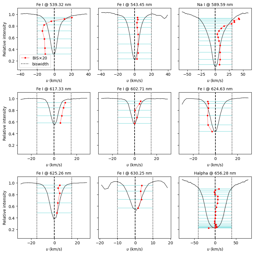
We provied a list of biswidth in the example above. These values were chosen after inspecting each of the selected lines. Remember to carefully select this parameter when running a similar analysis, as wiggles around the continuum might confuse the bisector function. By construction, the bisector function attempts to prevent that issue by removing 5% of the line profile near the continuum from the line bisector calculation.

We can now loop over the individual line profiles and call the calc_bis function. The code below illustrates the line profiles computed for the list of individual lines defined above.

Show code cell source Hide code cell source

ncols = 3
nrows = int(np.ceil(len(lambda0)/ncols))

fig, grid = plt.subplots(nrows, ncols, figsize=(9,9), sharey=True)
axes = grid.flatten()

vspan = np.zeros(len(lambda0))
vspan_std = np.zeros(len(lambda0))
vtop = np.zeros(len(lambda0))
vbottom = np.zeros(len(lambda0))
for id in range(len(lambda0)):
    # Get the line bisector and velocity span. 
    # Note that fullOutput is set to true in this example.
    vspan[id], vspan_std[id], vtop[id], vbottom[id], bisector, int_lvl = profs[id].calc_bis(
        cog=0.0, Ic=1.0, biswidth=biswidth[id], fullOutput=True)

    #### Plot ###
    axes[id].errorbar(profs[id].vel, profs[id].specI, yerr=profs[id].specSigI, 
                      c='k', lw=0.8, zorder=1)
    scale_bisector = 20.0 # arbitrary scale for plotting bisector
    axes[id].plot(bisector*scale_bisector, int_lvl, 'r.-', lw=0.5, zorder=2, 
                  label=r'BIS$\times {:.0f}$'.format(scale_bisector))
    axes[id].axvline(biswidth[id], c='k', ls=':', zorder=0, label='biswidth')
    axes[id].axvline(-biswidth[id], c='k', ls=':', zorder=0)
    axes[id].axvline(0.0, c='k', ls='--', zorder=0)
    axes[id].hlines(int_lvl, xmin=-biswidth[id], xmax=biswidth[id], 
                    alpha=0.33, color='c', zorder=0)
    axes[id].set_title('{:} @ {:1.2f} nm'.format(line_ref[id], lambda0[id]), 
                       fontsize='medium')
    axes[id].set_xlabel(r'$\upsilon$ (km/s)', fontsize='medium')
    if id == 0:
        axes[id].legend()

for id in range(nrows):
    grid[id,0].set_ylabel(r'Relative intensity', fontsize='medium')

for id in range(len(lambda0), len(axes)):
    axes[id].set_axis_off()

plt.tight_layout()