How to calculate the longitudinal field and False Alarm Probability#
The calculation of the longitudinal magnetic field (\(B_{z}\)) from a Stokes V line profile is done using:
where \(I(v)\) and \(V(v)\) are the continuum normalized \(I/I_c\) and \(V/I_c\), \(v\) is the velocity relative to the center of the line, and
When calculating \(B_{z}\) from an LSD profile, the rest wavelength of the line (\(\lambda_o\)) and effective Landé factor (\(g_\mathrm{eff}\)) should be the normalizing values used in the LSD calculation.
Note that the calc_bz function of the LSD class presented here requires \(\lambda_o\) to be given in nanometers.
The False Alarm Probability (FAP) of a signal in Stokes V and the null profile is also computed over the same velocity range used in the \(B_z\) calculation. The FAP is the p-value for the probability that the observed Stokes V, or null, profile is consistent with just noise. More specifically, it is the probability that a model consisting of a flat line is consistent with the observations, based on \(\chi^2\). When reporting a detection of a signal based on the FAP, typically:
For a definitive detection, FAP < \(10^{-4}\)
For a marginal detection, FAP < \(10^{-2}\)
Although different sources may use slightly different thresholds, it can be helpful to adopt more conservative criteria when dealing with large numbers of stars.
1. Example with one LSD profile#
First import specpolFlow and any other packages
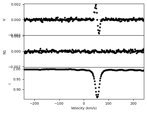
We load an example LSD profile (SampleLSD.lsd) and use the built-in plotting routine to visualize the Stokes V, null, and I profiles.
lsd = pol.read_lsd('CalculateBz_tutorialfiles/SampleLSD.lsd')
fig, ax = lsd.plot(figsize=(5,4))

To calculate Bz, we call the calc_bz function of the LSD object. The result is returned as a Python dictionary.
When using calc_bz you must provide the effective Landé factor (geff) and rest wavelength (lambda0) for the calculation. In general, these should be the normalizing values used for calculating the LSD profile.
Note
In LSD profiles that do not have a Null2 column, the LSD class replaces N2 with zeros, which means that the N2 Bz will also be set to zero.
1.1 Using the auto-normalization and auto-cog calculations#
In this example, we will use the automatic methods to renormalize the continuum of the LSD profile from the Stokes I (norm='auto') and compute the center of the line (the ‘center-of-gravity’ or cog) by using Stokes I only (cog='I').
To do so, we set the velrange option to [0.0, 100].0:
The data inside of this velocity range is used to calculate the center-of-gravity (cog) of the profile
The data outside of this velocity range is used to calculate the continuum level.
If we had not set the velrange keyword, the full range would have been be used for both calculations, although this usually produces less accurate results.
There are a few options for alternative ways of calculating the cog, in the calc_bz docs.
We also set the bzwidth keyword to specify the velocity range around the cog (i.e. relative to the line center) that will then be used to compute \(B_z\).
Note
The bzwidth can be set to a single float (for example, bzwidth=25.0 mean 25 km s\(^{-1}\) on each side of the cog). The bzwidth can also be set to a 2-item tuple or array (for example, bzwidth=(10.0, 25.0) mean 10 km s\(^{-1}\) on the blue side of the cog and 25 km s\(^{-1}\) on the red side of the cog). Usually the integration range in the \(B_z\) calculation should be symmetric about the line center, so bzwidth should usually be a single value.
If bzwidth is not defined, then the velrange is used to compute \(B_z\), which can be useful for specifying velocities in absolute units rather than relative to line center. (If both bzwidth and velrange are not defined, then the whole range is used - but avoid this!).
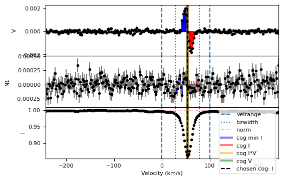
Combining these options and using plot=True to generate a figure gives us:
Bz, fig = lsd.calc_bz(cog='I', norm='auto',
                      geff=1.2, lambda0=500.0,
                      velrange=[0.0, 100.0], bzwidth=25.0,
                      plot=True, figsize=(6,4))
using AUTO method for the normalization
  using the median of the continuum outside of the line

The diagnostic figure above shows a few useful things:
The dashed vertical lines show the values of
velrange.The dotted vertical lines show the values of
bzwidth.The dashed horizontal line shows the value of the continuum level (
Icin the legend)The code always computes all of the automatic options for the cog. They are indicated by the vertical thick solid lines with the colors indicated by the legend.
The cog that you have selected (one of the automatic values or a user-defined value as discussed below) is shown in dashed black vertical line.
As you can see in the equation, \(B_z\) is related to the area under the curve of “Stokes V multiplied by (\(v-\mathrm{cog}\))”. In the graph, we show the area under the curve Stokes V only on each side of the cog. Note that this is only a guide.
The results are returned as a dictionary. You can see the results by printing it and accessing any value by its keyword:
print(Bz)
print('Bz = ', Bz["V bz (G)"], '+/-', Bz["V bz sig (G)"])
{'V bz (G)': 94.17678426512535, 'V bz sig (G)': 6.2520241712455595, 'V FAP': 0.0, 'N1 bz (G)': 4.858516305698941, 'N1 bz sig (G)': 6.122939627225724, 'N1 FAP': 0.76106309449015, 'N2 bz (G)': 0.0, 'N2 bz sig (G)': 0.0, 'N2 FAP': 0.0, 'norm_method': 'auto', 'norm': 0.99703, 'cog_method': 'I', 'cog': 53.3592394550717, 'int. range start': 28.3592394550717, 'int. range end': 78.3592394550717}
Bz =  94.17678426512535 +/- 6.2520241712455595
Tip
The dictionary returned by calc_bz can be directly converted to a Pandas dataframe. This can be convenient for saving or displaying results.
pd.DataFrame(data=[Bz]).style
| V bz (G) | V bz sig (G) | V FAP | N1 bz (G) | N1 bz sig (G) | N1 FAP | N2 bz (G) | N2 bz sig (G) | N2 FAP | norm_method | norm | cog_method | cog | int. range start | int. range end | |
|---|---|---|---|---|---|---|---|---|---|---|---|---|---|---|---|
| 0 | 94.176784 | 6.252024 | 0.000000 | 4.858516 | 6.122940 | 0.761063 | 0.000000 | 0.000000 | 0.000000 | auto | 0.997030 | I | 53.359239 | 28.359239 | 78.359239 |
The function reports \(B_z\), the uncertainty on \(B_z\), and the FAP, calculated with Stokes V (V bz (G), V bz sig (G), V FAP), and then the same quantities calculated using the nulls in place of Stokes V (N1 and N2).
The function reports the computed values for the continuum level (norm) and the center of gravity value (cog). It also returns the exact bounds that were used for the computation of \(B_z\) and FAP. For example, here, we set Bzwidth to be 25 km s\(^{-1}\) on each side of the cog, and the computed cog was 53.36 km s\(^{-1}\). Therefore, 25 km s\(^{-1}\) on each side of this cog will correspond to a velocity range of 28.36 km s\(^{-1}\) to 78.36 km s\(^{-1}\).
1.2 Using user-defined normalization and cog#
In the previous example, we used automatic methods to calculate the continuum normalization and the cog.
In some circumstances, you might not want to use the automatic methods. Perhaps you have already calculated your cog and your normalization. Perhaps you are trying to reproduce someone else’s results. Perhaps the line shape is complicated, and the automatic methods do not give a good result.
In this, we can simply set cog=float and norm=float.
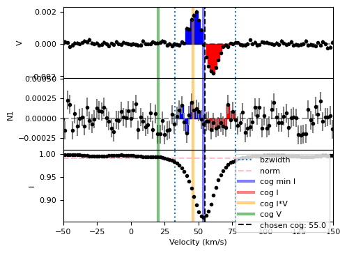
For example below, let’s say that we have already computed \(v_\mathrm{rad}\) and know that the continuum should be at 0.99.
We will add one little thing: let’s say you have already measured the line broadening and would like the \(B_z\) computation to be done in a range corresponding to \(1.5\times v\sin i\).
# Bz calculation using manual cog selection
vsini = 15.0
vrad = 55.0
Ic=0.99

lsd = pol.read_lsd('CalculateBz_tutorialfiles/SampleLSD.lsd')

Bz, fig = lsd.calc_bz(cog=vrad, bzwidth=1.5*vsini, norm=Ic,
                      plot=True, figsize=(5,4))

for item in fig.get_axes():
    item.set_xlim(-50,150)

pd.DataFrame(data=[Bz]).style
using given norm value
| V bz (G) | V bz sig (G) | V FAP | N1 bz (G) | N1 bz sig (G) | N1 FAP | N2 bz (G) | N2 bz sig (G) | N2 FAP | norm_method | norm | cog_method | cog | int. range start | int. range end | |
|---|---|---|---|---|---|---|---|---|---|---|---|---|---|---|---|
| 0 | 110.831819 | 6.014489 | 0.000000 | 7.256635 | 5.880429 | 0.722025 | 0.000000 | 0.000000 | 0.000000 | 0.990000 | 0.990000 | 55.000000 | 55.000000 | 32.500000 | 77.500000 |

As you can see, the label in the legend for the dashed vertical black line now reflects the value of the cog that was specified.
Also, you will note that we did not define a velrange. This was uncesesary, as we are not using the automated methods for neither the cog nor the continuum normalization.
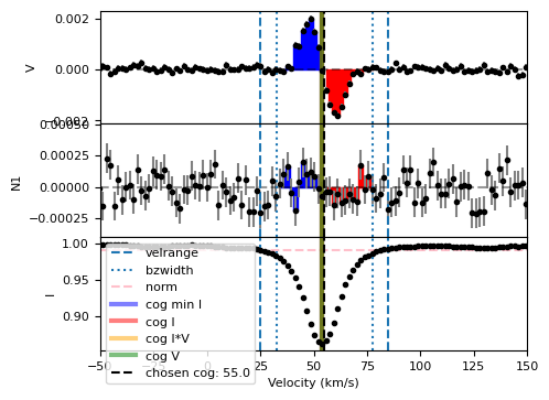
This said, if you would like to see how your choice for cog compares with the automated methods (which are always displayed in the diagnostic plot), then you could set an additional velrange. In the example below, we set it to be \(2\times v\sin i\) on each side of our pre-computed radial velocity.
Bz, fig = lsd.calc_bz(cog = vrad, bzwidth = 1.5*vsini, norm=Ic,
                      velrange=[vrad-2*vsini, vrad+2*vsini],
                      plot = True, figsize=(5,4))

for item in fig.get_axes():
    item.set_xlim(-50,150)
using given norm value

2. Calculating Bz for multiple LSD profiles.#
When processing multiple LSD profiles, particularly multiple observations of the same star, it can be efficient to loop over a list of LSD profiles. Then Bz can be calculated for each profile, by calling calc_bz inside the loop. In this example we consider LSD profiles from two different stars. We compute Bz and save the results for each observation into a list, converting the list of dictionaries into Pandas dataframe. Then, we add a column to the dataframe with the name of the stars.
The observed stars have different radial velocities and line widths. So we need to change velrange and bzwidth for each input file. If the observations are all for one single star, these values can usually be constant.
files = ['CalculateBz_tutorialfiles/SampleLSD.lsd',
         'CalculateBz_tutorialfiles/SampleLSD2.lsd']
velrange_list = [[10., 95.],
                 [-10., 55.]]
bzwidth_list = [25., 20.]

Bz_list = []
for i, file in enumerate(files):
    # load the LSD profile
    lsd = pol.read_lsd(file)
    # calculate Bz, this time without plotting each profile
    Bz = lsd.calc_bz(cog='I', velrange=velrange_list[i],
                     bzwidth=bzwidth_list[i],
                     geff=1.2, lambda0=500.0, plot=False)
    Bz_list += [Bz]
Bz_table = pd.DataFrame(Bz_list)

# let's add a column to the table with the filename
Bz_table.insert(0, 'Filename', files, True)
# and you can add a column to the table with more descriptive names
names = ['star 1', 'star 2']
Bz_table.insert(0, 'Observation', names, True)

# display the table
Bz_table.style
using AUTO method for the normalization
  using the median of the continuum outside of the line
using AUTO method for the normalization
  using the median of the continuum outside of the line
| Observation | Filename | V bz (G) | V bz sig (G) | V FAP | N1 bz (G) | N1 bz sig (G) | N1 FAP | N2 bz (G) | N2 bz sig (G) | N2 FAP | norm_method | norm | cog_method | cog | int. range start | int. range end | |
|---|---|---|---|---|---|---|---|---|---|---|---|---|---|---|---|---|---|
| 0 | star 1 | CalculateBz_tutorialfiles/SampleLSD.lsd | 94.584944 | 6.278508 | 0.000000 | 4.848727 | 6.148771 | 0.761063 | 0.000000 | 0.000000 | 0.000000 | auto | 0.996810 | I | 53.617944 | 28.617944 | 78.617944 |
| 1 | star 2 | CalculateBz_tutorialfiles/SampleLSD2.lsd | 32.111990 | 10.562343 | 0.002714 | -0.484883 | 10.561599 | 0.845782 | 0.000000 | 0.000000 | 0.000000 | auto | 0.995230 | I | 22.428587 | 2.428587 | 42.428587 |
With the results in a Pandas dataframe (see the Pandas documentation), we can do several things easily. We can save the table to a file (in this example a text .csv). We can also extract specific columns or rows from the table.
# save the table to a file
Bz_table.to_csv('CalculateBz_tutorialfiles/BzTable.csv')
# get a row for one observation only:
star2 = Bz_table[Bz_table['Observation']=='star 2']
star2.style
| Observation | Filename | V bz (G) | V bz sig (G) | V FAP | N1 bz (G) | N1 bz sig (G) | N1 FAP | N2 bz (G) | N2 bz sig (G) | N2 FAP | norm_method | norm | cog_method | cog | int. range start | int. range end | |
|---|---|---|---|---|---|---|---|---|---|---|---|---|---|---|---|---|---|
| 1 | star 2 | CalculateBz_tutorialfiles/SampleLSD2.lsd | 32.111990 | 10.562343 | 0.002714 | -0.484883 | 10.561599 | 0.845782 | 0.000000 | 0.000000 | 0.000000 | auto | 0.995230 | I | 22.428587 | 2.428587 | 42.428587 |
# get the columns for the Stokes V Bz value, and its uncertainty
Bz_V = Bz_table[['V bz (G)', 'V bz sig (G)']]
Bz_V.style
| V bz (G) | V bz sig (G) | |
|---|---|---|
| 0 | 94.584944 | 6.278508 |
| 1 | 32.111990 | 10.562343 |
# turn this into a numpy array
arr_Bz_V = Bz_V.to_numpy()
print(arr_Bz_V)
[[94.58494375  6.27850841]
 [32.11198956 10.56234263]]
