How to use Spectrum objects#
SpecpolFlow provides a python class that holds a Spectrum object. These objects contain the basic data for a spectroscopic or spectropolarimetric observation.
A Spectrum object contains the following data arrays:
wl - wavelengths
specI - Stokes I spectrum
specV - polarized spectrum, usually Stokes V
specN1 - the first polarimetric null spectrum
specN2 - the second polarimetric null spectrum
specSig - the formal uncertainties, which apply to the all spectra.
header - the text in the header of a .s file
For an observation with just an intensity spectrum (no polarization), the specV, specN1, and specN2 arrays will all be zeros.
First import specpolFlow and any other packages
In this tutorial, we use the UPENA normalized spectrum (IndividualLine_tutorialfiles/1423137pn.s) of the active cool star BP Tau.
How to load and save a Spectrum from a ‘.s’ file#
To load in a spectrum in .s format, we can use the read_spectrum function.
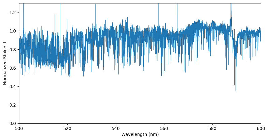
spec = pol.read_spectrum('IndividualLine_tutorialfiles/1423137pn.s')

# Make a figure of Stokes I over a specified region
fig, ax = plt.subplots(1, 1, figsize=(10,5))
ax.plot(spec.wl, spec.specI, lw=0.5)
ax.set_ylim(0.0, 1.3)
ax.set_xlim(500.0, 600.0)
ax.set_xlabel('Wavelength (nm)')
ax.set_ylabel('Normalized Stokes I')
plt.show()
If the ‘.s’ file has a text header, it will be available from the header property of the Spectrum object:
print(spec.header)
None
As you can see here, since the file did not have a header, the spec.header is set to None. (Note, this uses the special Python value None, not the text “None”).
A Spectrum object can be saved in a text ‘.s’ format with the spectrum.save class function.
In the example below, we will add a header to the Spectrum object and save it.
spec.header = 'Spectrum for star BP Tau'

spec.save('Output/Spectrum.s', saveHeader = True)
# saveHeader = True is the default
# saveHeader = False will skip the '.s' 2-line header when writing the file
Note
The Spectrum class supports 3 types of ‘.s’ file format
Polarimetric spectrum with 6 columns
Spectroscopic spectrum with 3 columns (Wavelength, Flux, uncertainty): in this case the spectrum.specV, spectrum.N1, spectrum.N2 will be set to zero
Spectroscopic spectrum with 2 columns (Wavelength, Flux): in this case spectrum.specSig, spectrum.specV, spectrum.N1, spectrum.N2 will be set to zero
The Spectrum.save function will save the spectrum in a 2, 3, or 6 column format if it detects columns that are strictly filled with zeros.
If you have a spectrum as columns in a text file, but it doesn’t match one of the standard 2, 3, or 6 column ‘.s’ formats, you can still use the read_spectrum function by specifying including the usecols argument. With usecols you can specify which columns are the wavelength, flux (Stokes I), and optionally other parameters. The columns count from 0, and the order that the columns are specified in corresponds to which parameter that column is used for. The order of things specified is: wavelength, Stokes I, Stokes V, null 1, null 2, and uncertainties. If a parameter isn’t given, or a column value of -1 is given, then the parameter is set to zeros. For example usecols=(0,3) reads wavelength from the 1st column, flux from the 4th column and leaves everything else as zeros. usecols=(0,3,2) reads wavelength from the 1st column, flux from the 4th column, and Stokes V from the 3rd column. usecols=(0, 1, -1, -1, -1, 4) reads wavelength from the 1st column, flux from the 2nd column, uncertainties from the 5th column, and leaves everything else as zeros.
# Read just two specified columns from a text file
# In this example we save the 5th column as Stokes I
# (even though that is really a null spectrum with just noise in this file)
spec_0_4 = pol.read_spectrum('IndividualLine_tutorialfiles/1423137pn.s', usecols = (0,4))
# To check, lets print the average and standard deviation of what we read in
print(np.average(spec_0_4.specI), np.std(spec_0_4.specI))
-0.0066444952597331484 0.10913875859554811
How to Doppler shift#
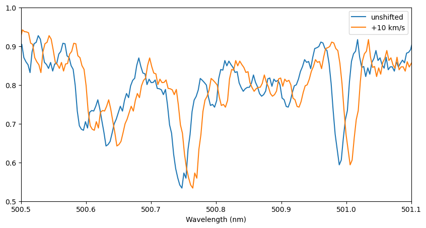
A Spectrum object has a function doppler_shift, which Doppler shifts the spectrum by a velocity given in km/s. In this function the positive radial direction is going away from the observer, so a positive velocity produces a redshift.
# Doppler shift a spectrum by 10 km/s
spec_10kms = spec.doppler_shift(10.0)

# Plot a comparison of the results
fig, ax = plt.subplots(1, 1, figsize=(10,5))
ax.plot(spec.wl, spec.specI, label='unshifted')
ax.plot(spec_10kms.wl, spec_10kms.specI, label='+10 km/s')
ax.set_xlim(500.5, 501.1)
ax.set_ylim(0.5, 1.0)
ax.set_xlabel('Wavelength (nm)')
ax.legend()
plt.show()
You can do the same thing by modifying the wavelength array of the Spectrum object directly, like:
spec.wl = spec.wl + spec.wl*10.0/2.9979e5
the doppler_shift function is just a bit more convenient.
Most spectrographs provide wavelengths in air, but some provide wavelengths in vacuum (usually when the spectrograph itself is in a vacuum chamber!). Usually it is ok to just work with wavelengths in air, or just work with wavelengths in vacuum. If you find you need to convert from one to the other, the conversion isn’t exactly a Doppler shift. Instead, the Spectrum class has vacuum_to_air and air_to_vacuum functions you can use.
How to use indexing and concatenation#
A Spectrum object can be sliced and indexed using normal Python list indexing and Numpy advanced indexing.
spec = pol.read_spectrum("IndividualLine_tutorialfiles/1423137pn.s")

print('The spectrum has {} datapoints'.format(len(spec)))

print('The maximum wavelength is {} nm'.format(spec.wl[-1]))

# Get the portion of a spectrum with wavelengths above 600 nm, and then check the first wavelength value
cut_spectrum = spec[spec.wl > 600.0]
print(cut_spectrum[0].wl)

# Get the portion of a spectrum in a specific wavelength range, and then check the first and last values
slice_650_663 = spec[(spec.wl > 650.0) & (spec.wl < 663.0)]
print(slice_650_663[0].wl, slice_650_663[-1].wl)
The spectrum has 213542 datapoints
The maximum wavelength is 1048.0382 nm
600.0012
650.0032 662.9992
You can assign values to the individual arrays that are part of a Spectrum object, for example like this:
spec.specI[0:7000] = 1.0
spec.specV[0:7000] = 0.0
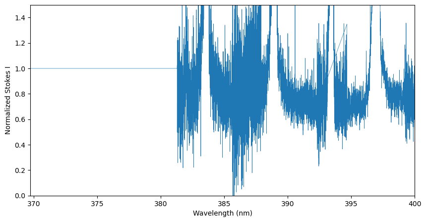
For a slightly more advanced example, we illustrate how one can assign a Spectrum object to a slice of another Spectrum object. Here, we replace a section of the spectrum with ones for the intensity and zeros for the polarization.
# Create a new Spectrum object with 7000 datapoints
n = 7000
replace = pol.Spectrum(spec.wl[0:n], np.ones(n), # wl and specI
                       np.zeros(n), np.zeros(n), np.zeros(n), # specV, specN1, and specN2
                       np.ones(n)) # specSig

# Overwrite a portion of an existing Spectrum object
spec[0:n] = replace

# Make a figure of Stokes I
fig, ax = plt.subplots(1, 1, figsize=(10,5))
ax.plot(spec.wl, spec.specI, lw=0.5)
ax.set_ylim(0.0, 1.5)
ax.set_xlim(min(spec.wl), 400.0)
ax.set_xlabel('Wavelength (nm)')
ax.set_ylabel('Normalized Stokes I')
plt.show()
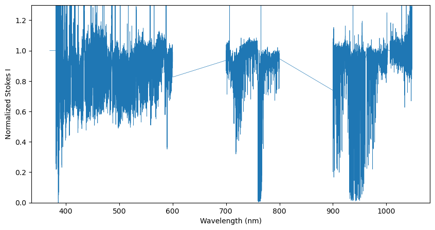
We can also concatenate mutiple Spectrum objects using the Spectrum.concatenate class function.
In the example below, we create three new Spectrum objects by slicing spec, and we then join them together
spec1 = spec[spec.wl < 600.0]
# You can combined criteria using & and brackets:
spec2 = spec[(spec.wl > 700.0) & (spec.wl < 800.0)]
# Or you can use numpy's logic functions:
spec2 = spec[np.logical_and(spec.wl > 700.0, spec.wl < 800.0)]
spec3 = spec[spec.wl > 900.0]

# Join the pieces of spectrum together
spec_cat = spec1.concatenate([spec2, spec3])

# Make a figure of Stokes I
fig, ax = plt.subplots(1, 1, figsize=(10,5))
ax.plot(spec_cat.wl, spec_cat.specI, lw=0.5)
ax.set_ylim(0.0, 1.3)
ax.set_xlabel('Wavelength (nm)')
ax.set_ylabel('Normalized Stokes I')
plt.show()
How to extract and merge spectral orders for echelle spectra#
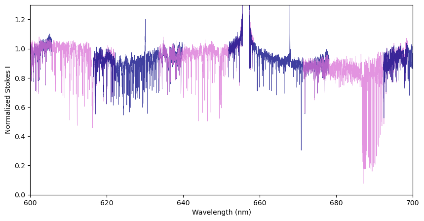
Some spectra will contain order-overlaps (wavelength regions that were recorded twice by an echelle spectrograph, in two different orders). In the .s format, the wavelength column goes backward at the edges of the overlaps.
In the figure below, we illustrate these overlap regions by color-coding the different spectral orders. This example uses the Spectrum.get_orders class function to make individual Spectrum objects for each echelle order.
spec = pol.read_spectrum("IndividualLine_tutorialfiles/1423137pn.s")

# Get the individual spectral orders
orders = spec.get_orders()
order_color=['orchid', 'navy']

# Make a figure of Stokes I
fig, ax = plt.subplots(1, 1, figsize=(10,5))
for i, order in enumerate(orders):
    ax.plot(order.wl, order.specI, lw=0.5, c=order_color[i % 2], alpha=0.75)
ax.set_ylim(0.0, 1.3)
ax.set_xlim(600.0, 700.0)
ax.set_xlabel('Wavelength (nm)')
ax.set_ylabel('Normalized Stokes I')
plt.show()
If you are only interested in spectral orders around a specific wavelength or range, you can use the Spectrum.get_orders_in_range class function. This will get only special orders that include the wavelength range requested and return them as a list of Spectrum objects.
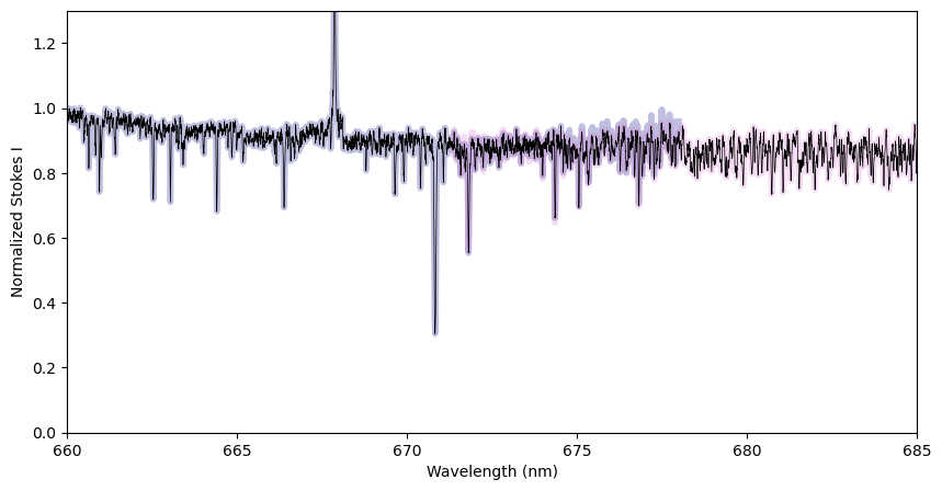
For some kinds of analysis, it is important to remove the order overlap regions, so that the wavelength increases continuously and there are no near-duplicate pixels. SpecpolFlow provides two methods to deal with all of the order overlaps all at once.
Tip
If you are interested in a specific spectral line and need to consider the order merging process more carefully, have a look at the How analyze individual spectral lines tutorial.
We here use the ‘trim’ method of the Spectrum.merge_orders function, which keeps a fraction of the overlap in each adjacent order, with the proportion set according to the ‘midpoint’ keyword. This is the simplest method and can be helpful if the continuum normalization is poor near order edges.
# Using the Spectrum class function to create a Spectrum object
# with the overlap merged trimmed in the middle of the overlap
spec_merged = spec.merge_orders(mode='trim', midpoint=0.5)

# If you'd like to save the result to a file, you can use the
# save class-function: spec_merged.save('spectrum_merged.s')

# Make a figure of Stokes I
fig, ax = plt.subplots(1, 1, figsize=(10,5))
for i, order in enumerate(orders):
    ax.plot(order.wl, order.specI, lw=4, c=order_color[i % 2], alpha=0.25)
ax.plot(spec_merged.wl, spec_merged.specI, lw=0.5, c='k')
ax.set_ylim(0.0, 1.3)
ax.set_xlim(660.0, 685.0)
ax.set_xlabel('Wavelength (nm)')
ax.set_ylabel('Normalized Stokes I')
plt.show()
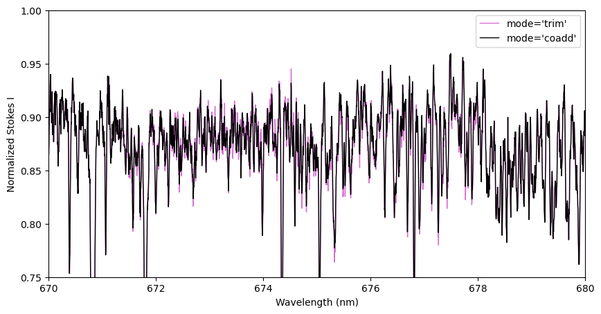
Alternatively, you can use the ‘coadd’ method, which tries to coadd pixels from the two orders in the overlap region. This essentially interpolates pixels from the second order onto the wavelengths of the first order before combining them. This optimizes the total S/N in the overlap region, but is vulnerable to systematic errors (e.g. poor normalization) in either spectral order.
# Merge spectral orders by coadding pixels
spec_merged2 = spec.merge_orders(mode='coadd')

# Compare the results from the two approaches to merging orders
fig, ax = plt.subplots(1, 1, figsize=(10,5))
ax.plot(spec_merged.wl, spec_merged.specI, lw=1.0, c='orchid', label="mode='trim'")
ax.plot(spec_merged2.wl, spec_merged2.specI, lw=1.0, c='k', label="mode='coadd'")
ax.set_ylim(0.75, 1.0)
ax.set_xlim(670.0, 680.0)
ax.set_xlabel('Wavelength (nm)')
ax.set_ylabel('Normalized Stokes I')
ax.legend()
plt.show()
How to coadd multiple spectra#
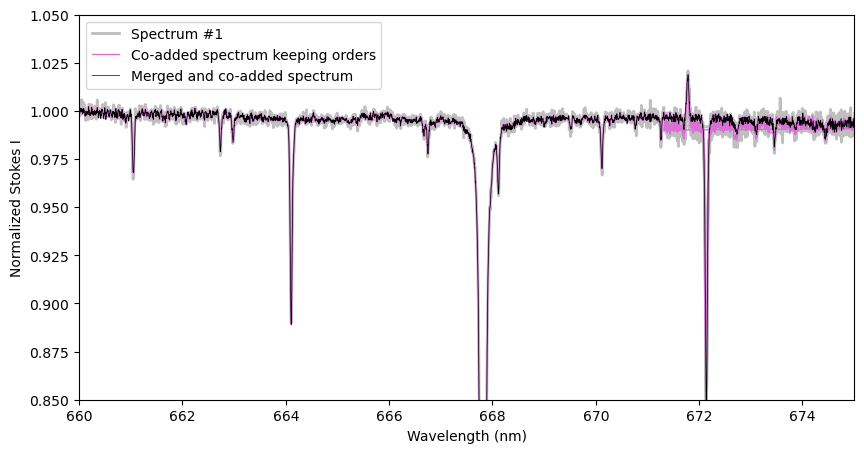
Sometimes you may have multiple spectra that you would like to average together, for example, a long ESPaDOnS observation that was split into multiple sequences to respect the integration time limit. You can use the Spectrum.coadd class function for this. This essentially averages spectra weighted by the error bars (really weighted by \(1/\sigma^2\)). Thus this needs valid error bars to work. The function interpolates the wavelengths of the observations onto the wavelength grid of the first spectrum (i.e. onto the wavelength grid of the Spectrum object calling the coadd function).
By default this function will split the function into separate orders (with the Spectrum.get_orders function), and then coadd each order individually. For this to work the spectra all need to have the same number of orders. This can be turned off by setting the argument byOrders=False, but if there are any overlapping regions in the spectrum (places where the wavelength jumps backwards), this will cause bad results in those regions! Alternatively, any spectral orders can be merged before running coadding by setting the flag mergeOrders='trim' or 'coadd' (see the Spectrum.merge_orders function for details on those flags).
Usually if you are working with unnormalized spectra it is safer to coadd them by order, and not merge the orders. This makes it easier to normalize them later. With well normalized spectra, coadding by order or merging orders are both reasonable approaches.
For this example, we will use 3 observations of the B-type star HD 46328:
# Reading the spectra
spec1 = pol.read_spectrum('../GetStarted/OneObservationFlow_tutorialfiles/hd46328_test_1.s')
spec2 = pol.read_spectrum('../GetStarted/OneObservationFlow_tutorialfiles/hd46328_test_2.s')
spec3 = pol.read_spectrum('../GetStarted/OneObservationFlow_tutorialfiles/hd46328_test_3.s')

# The coadd class-function might return an error if the uncertainty in the
# spectra are zero or negative (because of the weighting)
# Here, remove these 'bad pixels' by setting the uncertainty to infinity
# (so they will not contribute to the weighted average)
spec1.specSig[spec1.specSig <= 0.0] = np.inf
spec2.specSig[spec2.specSig <= 0.0] = np.inf
spec3.specSig[spec3.specSig <= 0.0] = np.inf

# co-adding the 3 spectra together
# (interpolating on the wavelength grid of the first spectrum)
spec_coadd = spec1.coadd([spec2, spec3])

# This star is more complicated: it's a pulsator with large radial velocity variations
# To optimally coadd we should apply a Doppler shift first, correcting for the pulsations
vrad = [12.0, 42.0, 16.0] #radial velocities, km/s
c = 2.99792458e5 #speed of light in km/s
spec1.wl = spec1.wl - spec1.wl*vrad[0]/c
spec2.wl = spec2.wl - spec2.wl*vrad[1]/c
spec3.wl = spec3.wl - spec3.wl*vrad[2]/c

# then coadd the Doppler shifted spectra
spec_coadd = spec1.coadd([spec2, spec3])

# alternatively, you can merge the spectral orders before coadding them, like this
spec_coadd_merged = spec1.coadd([spec2, spec3], mergeOrders='trim')

# Make a figure of Stokes I
fig, ax = plt.subplots(1, 1, figsize=(10,5))
ax.plot(spec1.wl, spec1.specI, lw=2, c='0.75', label='Spectrum #1')
ax.plot(spec_coadd.wl, spec_coadd.specI, lw = 1.0, c='orchid', label='Co-added spectrum keeping orders')
ax.plot(spec_coadd_merged.wl, spec_coadd_merged.specI, lw = 0.5, c='k', label='Merged and co-added spectrum')
ax.set_ylim(0.85, 1.05)
ax.set_xlim(660.0, 675.0)
ax.set_xlabel('Wavelength (nm)')
ax.set_ylabel('Normalized Stokes I')
ax.legend()
plt.show()
What if you don’t have the correct file type but you have the data?#
You may have a spectrum in a file type that we do not currently support and we don’t have a converter for it yet. If this is your situation, don’t despair! You can still load in spectrum data and create a Spectrum object from columns of data.
Below, I will naively load in the spectrum from a text file with numpy.
unknown_file = np.loadtxt('IndividualLine_tutorialfiles/1423137pn.s')
# Now you can use individual columns of your data to make your own Spectrum Object
wave = unknown_file[:,0]
flux = unknown_file[:,1]
err = unknown_file[:,5]
emptyarr = np.zeros_like(wave)
toto = pol.Spectrum(wave, flux, emptyarr, emptyarr, emptyarr, err)
# Make a figure of Stokes I over a specified region
fig, ax = plt.subplots(1, 1, figsize=(10,5))
ax.plot(toto.wl, toto.specI, lw=0.5)
ax.set_ylim(0.0, 1.3)
ax.set_xlim(500.0, 600.0)
ax.set_xlabel('Wavelength (nm)')
ax.set_ylabel('Normalized Stokes I')
plt.show()
This is the same plot from earlier in the tutorial. From here, you can treat your column-generated Spectrum object the same as if you had made it using pol.read_spectrum.
You can do the same thing with a FITS file, if you know the file format. You can use Astropy (astropy.io.fits) to read the file, and then take the arrays of data and store them in a Spectrum object like in the example above.