How to compute equivalent widths

The equivalent width (EW) of a line is a useful characteristic for describing the strength of a spectral feature. EWs have specific use cases in the study of different objects; for example, the EW of the Balmer alpha transition in T Tauri stars is used to classify them as being classical or weak-lined.

The equivalent width is essentially the area inside the line, between the line and the continuum. It is defined as

\[ \rm{EW} = \int \frac{F_c - F(\lambda)}{F_c} d\lambda,\]

where \(F_c\) is the continuum level, \(F(\lambda)\) is the observed line profile, and \(\lambda\) is the wavelength. For real observations with discrete pixels, this equation is usually discretized using numerical integration like

\[ \rm{EW} = \sum \frac{F_c - F_\lambda}{F_c} \Delta\lambda,\]

with a pixel spacing \(\Delta\lambda\). The EW and it’s uncertainty are typically reported in units of wavelength, although units of velocity can also be used, by dividing by the rest wavelength of the line and multiplying by the speed of light.

For this tutorial, we will use an observation of the T Tauri star BP T Tauri from ESPaDOnS, with an UPENA normalized spectrum (IndividualLine_tutorialfiles/1423137pn.s). First we import SpecpolFlow and any other packages.

Show code cell content

Hide code cell content

import specpolFlow as pol
import matplotlib.pyplot as plt
import pandas as pd

Using the Spectrum class calc_ew()

The simplest way to make an equivalent width calculation for a line in an observation is to use the calc_ew function of the Spectrum class. First, we read in the observed spectrum with read_spectrum. We then use the Spectrum merge_orders function to remove overlapping spectral orders, which can throw off the EW calculation. (Note that calc_ew does not expect overlapping echelle orders in the spectrum and will produce a warning message if it finds any overlap.) Next, we run the calc_ew function for that spectrum. We define lineRange as the wavelength range over which the integration is completed to calculate the EW. We also define contRange with a set of wavelength ranges that are used as continuum regions. contRange can be a List with two entries or a List of several Lists, each with two entries: a start and end wavelength for a continuum region. The final continuum level is calculated from the median of pixels in the continuum regions.

Here we set verbose=True to print out some information about the continuum level.

The calc_ew function returns a dictionary containing the results and some diagnostic information. The dictionary includes fields for the equivalent width 'EW' and its uncertainty 'EW sig', the continuum level used 'norm', and the integration range used from 'int. range start' to 'int. range end'.

spec = pol.read_spectrum("IndividualLine_tutorialfiles/1423137pn.s")
# remove order overlap by running the merge_orders function
spec = spec.merge_orders(mode='trim')
# calculate an equivalent width
ew_dict, figure = spec.calc_ew(lineRange=[643.81, 644.07],
                               contRange=[[643.60, 643.66],[643.77, 643.79],[644.1, 644.4]],
                               verbose=True)

# Print the full dictionary of results
print("a dictionary of results:")
print(ew_dict)

# Print just the most useful results
print("The equivalent width of this line is {:.4f} +/- {:.4f} nm.".format(ew_dict['EW'], ew_dict['EW sig']))
plt.show()

using AUTO method for the normalization
  using the median of the continuum outside of the line: 0.98812
a dictionary of results:
{'EW': 0.03758899800000324, 'EW sig': 0.00019497984684120867, 'norm_method': 'auto', 'norm': 0.98812, 'cog_method': 0.0, 'cog': 0.0, 'int. range start': 643.81, 'int. range end': 644.07}
The equivalent width of this line is 0.0376 +/- 0.0002 nm.

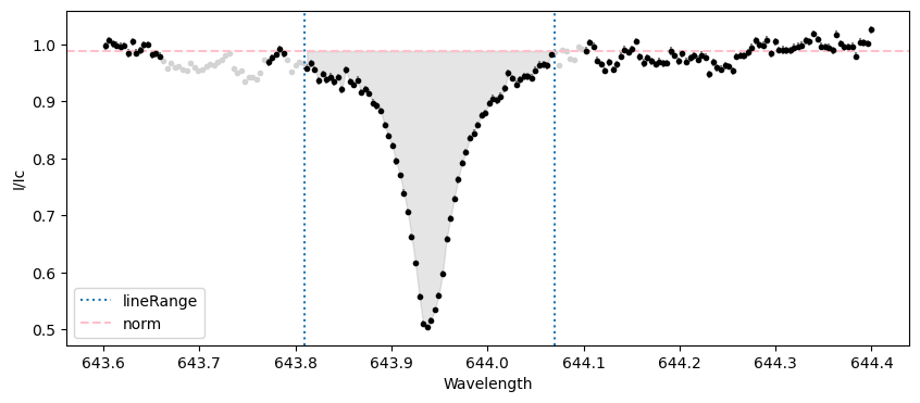
The dictionary of results can be loaded into a Pandas dataframe, for further analysis, or for formatted tables.

ew_dataframe = pd.DataFrame(data=[ew_dict], index=['obs1'])
# make a selection of the DataFrame using just the more useful columns
ew_table = ew_dataframe[['EW', 'EW sig', 'norm']]
ew_table.style  # show a table from this DataFrame

	EW	EW sig	norm
obs1	0.037589	0.000195	0.988120

By default the calc_ew function generates a diagnostic plot. The region used for the EW calculation is shaded, inside vertical lines. Regions used to estimate the continuum level are shown as outside the vertical lines as black points, and the continuum level is shown as a horizontal line. Pixels not used in the calculation are shown as grey points. If you don’t need the diagnostic plot (e.g. you are processing several observations) you can use plot=False.

ew_dict = spec.calc_ew(lineRange=[643.81, 644.07],
                       contRange=[[643.60, 643.66],[643.77, 643.79],[644.1, 644.4]],
                       verbose=False, plot=False)
print("The equivalent width of this line is {:.4f} +/- {:.4f} Å.".format(10*ew_dict['EW'], 10*ew_dict['EW sig']))

The equivalent width of this line is 0.3759 +/- 0.0019 Å.

The equivalent width calculation can also be applied to emission lines. This will produce a negative value, since this line is in emission (lines in absorption will be positive). Using positive values of EW for absorption lines and negative values of EW for emission lines is a convention we adopt here. But in other places positive values may be used for EWs of emission lines.

ew_dict, figure = spec.calc_ew(lineRange=[655.4, 657.2],
                               contRange=[[654.7, 655.1],[657.6, 658.1]])

print("The equivalent width of this line is {:.3f} +/- {:.3f} nm.".format(ew_dict['EW'], ew_dict['EW sig']))
plt.show()

The equivalent width of this line is -7.459 +/- 0.002 nm.

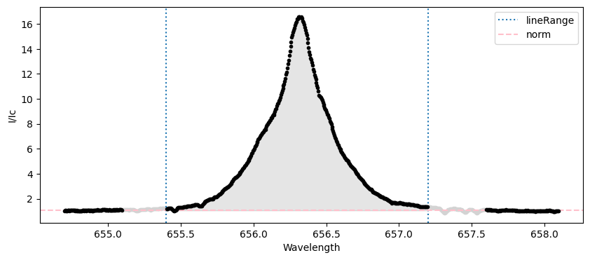
Part of the traditional definition of a Classical T Tauri star (as opposed to a weak-line T Tauri star) is that the equivalent width of H \(\alpha\) is greater than 10 Å (> 1 nm, or in this script < -1 nm). As we can see above, BP Tau seems like a Classical T Tauri star! For more information on BP Tau, check out this paper.

If you already know the continuum level, you can specify that with the norm parameter. If norm is set to a number, then contRange is not used. In this example we just fix the continuum to 1.0

ew_dict = spec.calc_ew(lineRange=[655.4, 657.2],
                       norm=1.0, plot=False)
print("The equivalent width of this line is {:.3f} +/- {:.3f} nm.".format(ew_dict['EW'], ew_dict['EW sig']))

The equivalent width of this line is -7.561 +/- 0.002 nm.

Using the LSD class calc_ew()

The LSD class also has a calc_ew function, which provides alternative input parameters that are very similar to the calc_bz function. This can be used to calculate EWs for LSD profiles. It can also be used to calculate EWs for individual lines in a real spectrum by using the Spectrum.individual_line function, to get one line from a Spectrum and convert it to an LSD object.

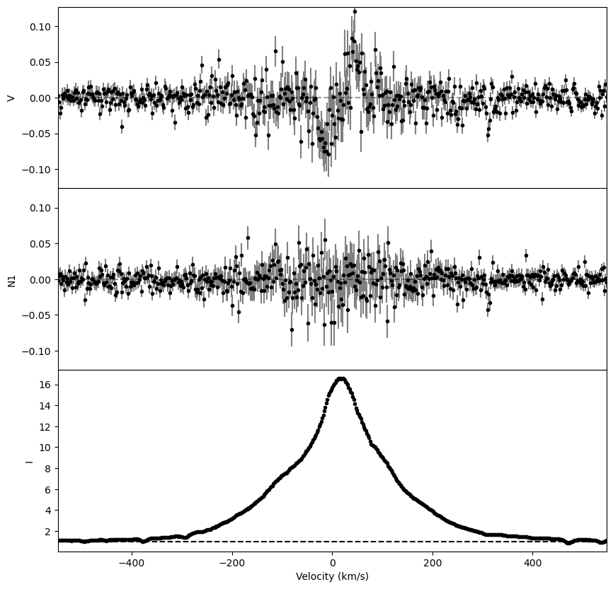
Below, we calculate the EW for the H \(\alpha\) line for our test star, BP T Tauri. We start be loading in the UPENA normalized spectrum, merging spectral orders, and extracting the line in question.

spec = pol.read_spectrum("IndividualLine_tutorialfiles/1423137pn.s")
# Make sure to remove order overlap before calculating EWs!
spec = spec.merge_orders(mode='trim')
# creating a line profile from just the Halpha line
prof_Halpha = spec.individual_line(lambda0 = 656.28, lwidth = 1.2)

fig, axes = prof_Halpha.plot()
axes[-1].axhline(1.0, color ='k', ls = '--') # add an extra line showing the continuum
plt.show()

calc_ew uses the above LSD object and the following parameters:

• cog - value or calculation method for the center of gravity; if not specified, will default to the cog of the Stokes I profile. This is only used for calculating the integration range, since ewwidth is relative to this value (for consistency with calc_bz).

• norm - calculation method for the continuum; the default here is auto, which uses the median of pixels outside velrange, but you can set it to a specific value by just setting it to that number.

• lambda0 - the wavelength of the line center. This is only used for converting the EW from km/s to wavelength units; if not given then the EW is in velocity units. If given, this should be the same lambda0 used to generate the LSD object.

• velrange - the velocity range used to determine the line center (pixels inside this range) and the continuum (pixels outside this range); if none is given, this will default to the full LSD object.

• ewwidth - the distance from the line center for the EW calculation; if one value is given, the range will be +/- this value from the center of the line, if two values are given, these will be the bounds of the integral. If no value is given, this will default to the velrange. Since this is an LSD object, the ewwidth is in velocity units (km/s).

• plot - bool; if True (default), the output will return a matplotlib figure.

This function returns a dictionary, which includes the equivalent width 'EW', its uncertainty 'EW sig', the continuum level used 'norm', the integration range used 'int. range start' to 'int. range end', and some other diagnostic information.

Below, we are specifying the lambda0 in nanometers so that the EW is returned in nanometers, if you specify lambda0 in Ångstroms the EW will be in Ångstrom, if lambda0 is not specified, the EW will be in km/s. In this example norm is set to fix the continuum at 1.0, ewwidth gives the velocity range for integration, and setting velrange to None means it defaults to the full LSD object above (which is ok since norm is a specified value, and velrange is only used for the cog estimate).

ew_dict, figure = prof_Halpha.calc_ew(lambda0=656.28, norm=1.0, velrange=None, ewwidth=400.0)

print("The equivalent width of this line is {:.2f} +/- {:.2f} nm.".format(ew_dict['EW'], ew_dict['EW sig']))
plt.show()

The equivalent width of this line is -7.55 +/- 0.00 nm.

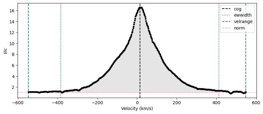
Here again, this value is negative since this line is in emission.

As a second example, we leave the EW in km/s and we do not specify the continuum level, but instead set velrange and let the continuum be estimated from the median of points outside velrange.

ew_dict = prof_Halpha.calc_ew(velrange=[-500.0,500.0], ewwidth=400.0, plot=False)
print("The equivalent width of this line is {:.1f} +/- {:.1f} km/s.".format(ew_dict['EW'], ew_dict['EW sig']))

The equivalent width of this line is -3352.6 +/- 0.7 km/s.

Violet to Red ratio calculation

Another useful quality is the V/R or Violet over Red ratio. This is the ratio of the equivalent width of the violet side of the line (shorter wavelength) to the red side of the line (longer wavelength). This can be calculated with the calc_V_R function, which is similar to using calc_ew.

This function is sensitive to the choice of the center-of-gravity of the line. This can be estimated automatically from the Stokes I (intensity) profile using cog='I', although this is only reliable for well behaved lines. Alternatively, this can be set using a radial velocity measured from other lines, which is what we use for this emission line example. Here we use the He I 5875 Å line, which is in emission for BP Tau. This line is asymmetric and redshifted from accretion.

profHe587 = spec.individual_line(lambda0 = 587.56, lwidth = 0.75)
rv = 15.5 # literature radial velocity in km/s 
V_R_dict, figure = profHe587.calc_V_R(ewwidth=110.0, cog=rv, norm = 'auto', velrange=[-120.0, 170.0], verbose=True)

print("The V/R of this line is {:.3f} +/- {:.3f} (relative to a cog {:.2f} km/s).".format(V_R_dict['V_R'], V_R_dict['V_R sig'], V_R_dict['cog']))
plt.show()

using AUTO method for the normalization
  using the median of the continuum outside of the line: 1.0076
The V/R of this line is 0.600 +/- 0.004 (relative to a cog 15.50 km/s).

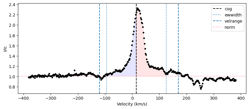
This metric is useful for checking the asymmetry of a line; for another tool that quantifies asymmetry, check out our Line Bisector tutorial!